1.37 Asymmetrical designs (Mediterranean molluscs)
Although a previous section has been devoted to the analysis of unbalanced designs, there are some special cases of designs having missing cells which deserve extra attention. Such designs are commonly referred to as asymmetrical designs, and consist essentially of there being different numbers of levels of a nested factor within each different level of an upper-level factor. Important examples include the asymmetrical designs that can occur in studies of environmental impact. Here, there might only be a single site that is impacted, whereas there might be multiple control (or unimpacted) sites (e.g., Underwood (1992) , Underwood (1994) , Glasby (1997) ). The reason for asymmetrical designs arising frequently in the analysis of environmental impacts is that it is generally highly unlikely that an impact site of a particular type (e.g., an oil spill, a sewage outfall, the building of a particular development, etc.) will be replicated, whereas there is often no reason not to include multiple replicate control sites (at a given spatial scale) against which changes at the (purportedly) impacted site might be measured (e.g., Underwood (1992) , Underwood (1994) ). On the face of it, the experimenter might consider that such a design presents a severe case of imbalance, where not all cells are filled. In actual fact, this is not really the case, because it is only the number of levels of the nested factor that are unequal, and actually all of the terms in the partitioning will be independent of one another, just as they would be in a balanced design.
An example of an asymmetrical design is provided by a study of subtidal molluscan assemblages in response to a sewage outfall in the Mediterranean ( Terlizzi, Scuderi, Fraschetti et al. (2005) ). The study area is located along the south-western coast of Apulia (Ionian Sea, south-east Italy). Sampling was undertaken in November 2002 at the outfall location and at two control or reference locations. Control locations were chosen at random from a set of eight possible locations separated by at least 2.5 km and providing comparable environmental conditions to those occurring at the outfall (in terms of slope, wave exposure and type of substrate). They were also chosen to be located on either side of the outfall, to avoid spatial pseudo-replication. At each of the three locations, three sites, separated by 80 - 100 m were randomly chosen. At each site, assemblages were sampled at a depth of 3 - 4 m on sloping rocky surfaces and n = 9 random replicates were collected (each replicate consisted of scrapings from an area measuring 20 cm × 20 cm), yielding a total of N = 81 samples. The experimental design is:
- Factor A: Impact versus Control (‘IvC’, fixed with a = 2 levels: I = impact and C = control).
- Factor B: Location (‘Loc’, random, nested in IvC with b = 2 levels nested in C and 1 level nested in I, labeled as numbers 1, 2, 3).
- Factor C: Site (random, nested in Loc(IvC) with c = 3 levels, labeled as numbers 1-9).
A schematic diagram (Fig. 1.52) helps to clarify this design, and why it is considered asymmetrical.

Fig. 1.52. Schematic diagram of the asymmetrical design for Mediterranean molluscs.
The data for this design are located in the file medmoll.pri in the ‘MedMoll’ folder of the ‘Examples add-on’ directory. As in Terlizzi, Scuderi, Fraschetti et al. (2005) , to visualise patterns among sites, we may obtain an MDS plot of the averages of samples at the site level. Go to the worksheet containing the raw data and choose Tools > Average > (Samples •Averages for factor: Site), then Analyse > Resemblance > (Analyse between: •Samples) & (Measure •Bray-Curtis), followed by Analyse > MDS.
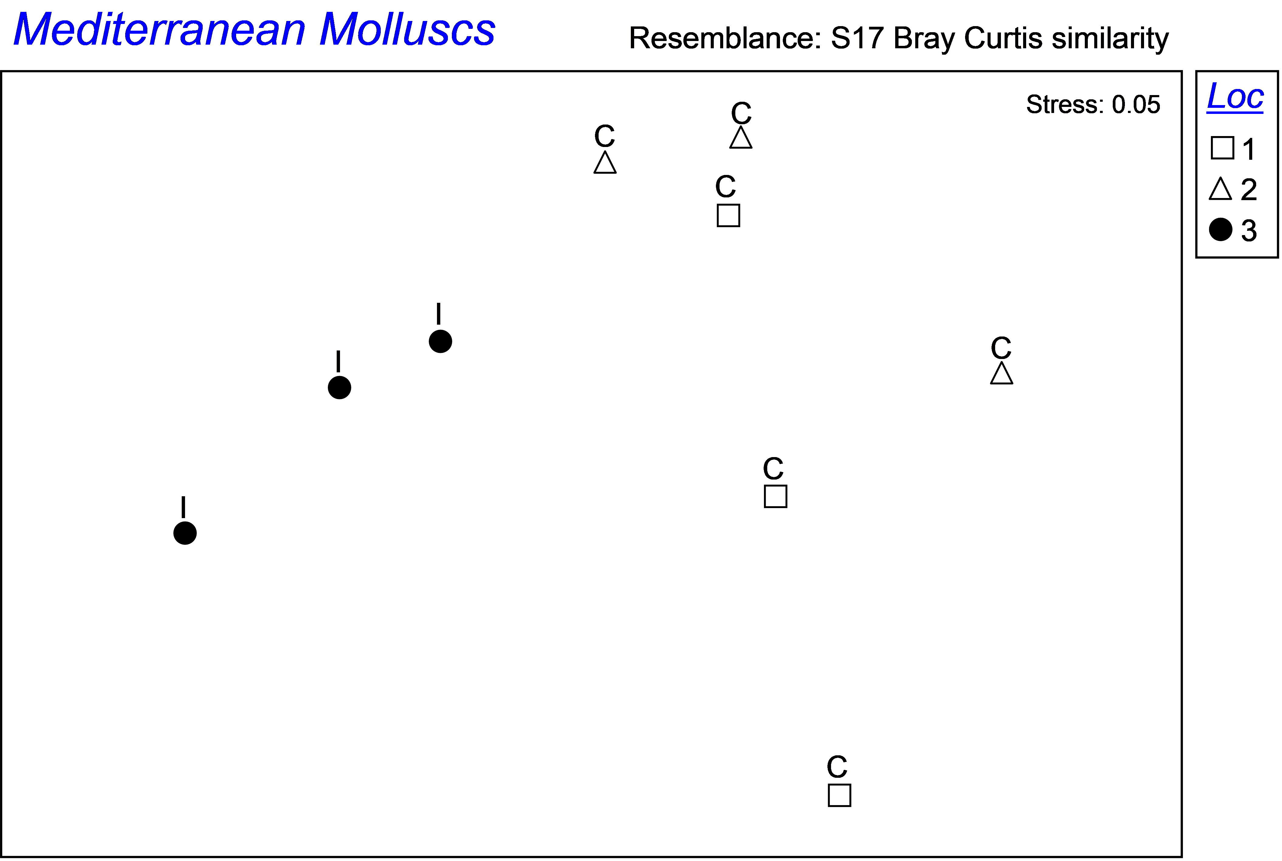
Fig. 1.53. MDS of site averages for Mediterranean molluscs, where I = impact and C = control locations.
There is apparent separation between the (averaged) assemblages at sites from the impact location compared to the controls on the MDS plot (Fig. 1.53), but to test this, we shall proceed with a formal PERMANOVA analysis. The difference, if any, between impact and controls must be compared with the estimated variation among control locations. Next, calculate a Bray-Curtis resemblance matrix directly from the original medmoll.pri raw data sheet (i.e., not the averaged data), then create a PERMANOVA design file according to the above experimental design, re-name the design file Asymmetric and proceed to run the analysis by choosing the following in the PERMANOVA dialog: (Design worksheet: Asymmetric) & (Test: •Main test) & (Sums of Squares •Type III (partial) ) & (Num. permutations: 9999) & (Permutation method •Permutation of residuals under a reduced model) & ($\checkmark$Do Monte Carlo tests) & ($\checkmark$Fixed effects sum to zero). For clarity in viewing these results, un-check (i.e. remove the $\checkmark$ from) the option to ‘Use short names’.
The results indicate that there is significant variability among sites, but variation among control locations is not detected over and above this site-level variability (i.e. the term ‘Loc(IvC)’ is not statistically significant P > 0.12, Fig. 1.54). There is also apparently a significant difference in the structure of molluscan assemblages at the impact location compared to the control locations (P(MC) = 0.036). Note that, in the absence of any replication of outfall (impact) locations, the only basis upon which location-level variability may be measured is among the (in this case only two) control locations. We should refrain from going overboard in the extent of our inferences here – it is inappropriate to place strong importance on an approximate MC P-value which relies on asymptotic theory (i.e. its accuracy gets better as sample size increases) yet was obtained using only two control locations and hence only 1 df in the denominator. Furthermore, of course, in the absence of any data from before the outfall was built, it is not possible to infer that the difference between the impact and the controls detected here was necessarily caused by the sewage outfall. It is also impossible to know whether this difference is something that has persisted or will persist in time. What we can say is that the molluscan assemblages at the outfall at the time the data were collected were indeed distinct from those found at the two control locations in the area sampled at that time, as observed in the MDS plot (Fig. 1.53).
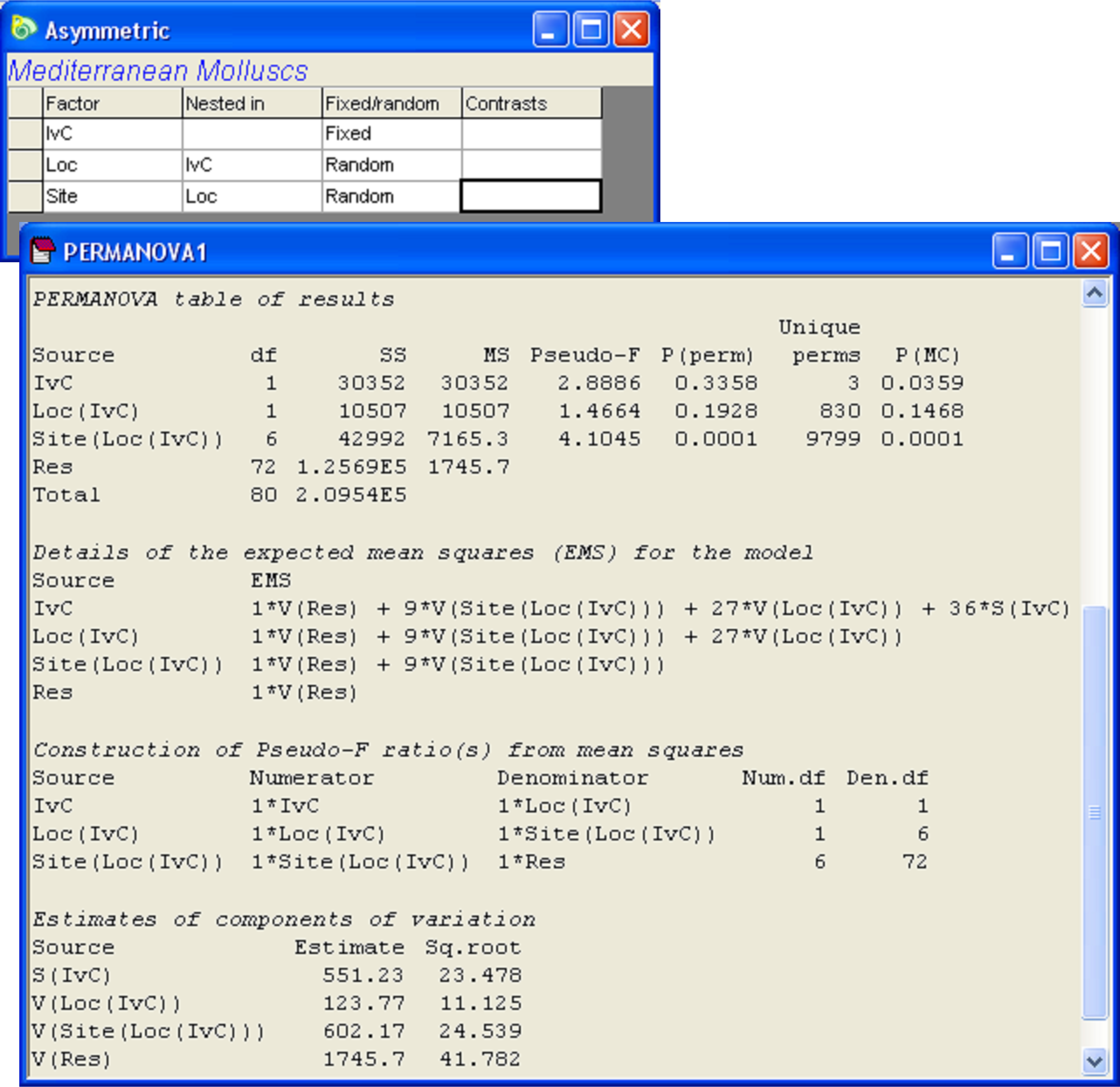
Fig. 1.54. PERMANOVA analysis of an asymmetrical design for mediterranean molluscs.
Asymmetrical designs such as this one have often previously been analysed and presented by partitioning overall location effects into two additive pieces: (i) the SS due to the contrast of the impact vs the controls and (ii) the SS due to the variability among the controls (e.g., Underwood (1994) , Glasby (1997) ). The reason for this has largely been because of the need for experimenters to utilise software to analyse these designs which did not allow for different numbers of levels of nested factors in the model. PERMANOVA, however, allows the direct analysis of each of the relevant terms of an asymmetrical design such as this, without having to run more than one analysis, and without any other special manipulations or calculations.
It is not necessary for the user to specify contrasts in PERMANOVA in order to analyse an asymmetrical design. It is essential to recognise the difference between the design outlined above, which is the correct one, and the following design, which is not:
- Factor A: Locations (fixed or random(?) with a = 3 levels and special interest in the contrast of level 3 (impact) versus levels 1 and 2 (controls),
- Factor B: Sites (random, b = 3 levels, nested in Locations)
Be warned! If an asymmetrical design is analysed using contrasts in PERMANOVA, then although the SS of the partitioning will be correct, the F ratios and P-values for some of the terms will almost certainly be incorrect! Note that the correct denominator MS for the test of ‘IvC’ must be at the right spatial scale, i.e. at the scale of locations, even though, in the present design (with only one impact location), our only measure of location-level variability comes from the control locations. Recall that a contrast, as a one-degree-of-freedom component partitioned from some main effect, will effectively use the same denominator as that used by the main effect (e.g., see the section Contrasts), which is not the logical choice in the present context. A clear hint to the problem underlying this approach is apparent as soon as we try to decide whether the ‘Locations’ factor should be fixed or random. It cannot be random, because the contrast of ‘IvC’ is clearly a fixed contrast of two states we are interested in. However, neither can it be fixed, because the control locations were chosen randomly. They are intended to represent a population of possible control locations and their individual levels are not of any interest in and of themselves. Once again, the rationale for analysing asymmetrical designs using contrasts in the past (and subsequently constructing the correct F tests by hand, see for example, Glasby (1997) ) was because software was not widely available to provide a direct analysis of the true design.
Although an asymmetrical design might appear to be unbalanced (and it is, in the sense that the amount of information, or number of levels, used to measure variability at the scale of the nested factor is different within different levels of the upper-level factor), it does not suffer from the issue of non-independence which was described in the section on Unbalanced designs. In fact, all of the terms in an asymmetrical design such as this are completely orthogonal (independent) of one another. So, it does not matter which Type of SS the user chooses, nor in which order the terms are fitted – the same results will be obtained. (This is easily verified by choosing to re-run the above analysis using, for example, Type I SS instead.)