5.7 Test by permutation (Anderson’s irises)

CAP can be used to test for significant differences among the groups in multivariate space. The test statistics in CAP are different from the pseudo-F used in PERMANOVA. Instead, they are directly analogous to the traditional classical MANOVA test statistics, so we will demonstrate them here in an example of classical canonical discriminant analysis (CDA). The data were obtained by Edgar Anderson ( Anderson (1935) ) and were first used by Sir R. A. Fisher ( Fisher (1936) ) to describe CDA (sometimes also called canonical variate analysis). Data are located in the file iris.priiris in the ‘Irises’ folder of the ‘Examples add-on’ directory. The samples here are individual flowers. On each flower, four morphometric variables were measured (in cm): petal length (PL), petal width (PW), sepal length (SL) and sepal width (SW). There were 150 samples in total, with 50 flowers belonging to each of 3 species: Iris versicolor (C), Iris virginica (V) and Iris setosa (S). Interest lies in using the morphometric variables to discriminate or predict the species to which individual flowers belong.

A traditional canonical discriminant analysis is obtained by running the CAP routine on the basis of a Euclidean distance matrix and manually choosing m = p, where p is the number of variables in the original data file. The first m PCO axes will therefore be equivalent to PCA axes and these will contain 100% of the original variation in the data cloud. Even if the original variables are on different units or scales, there is no need to normalise the data before proceeding with the CAP analysis, as this is automatically ensured by virtue of the fact that CAP uses orthonormal PCO axes. In some situations, the number of original variables will exceed (or come close to) the total number of samples in the data file (i.e., p approaches or exceeds N). In such cases, it is appropriate to use the leave-one-out diagnostics to choose m, just as would be done for non-Euclidean cases. An alternative would be to choose a subset of original variables upon which to base the analysis (by removing, for example, strongly correlated variables). Here, the usual issues and caveats regarding variable selection for modelling (see chapter 4) come into play.
 

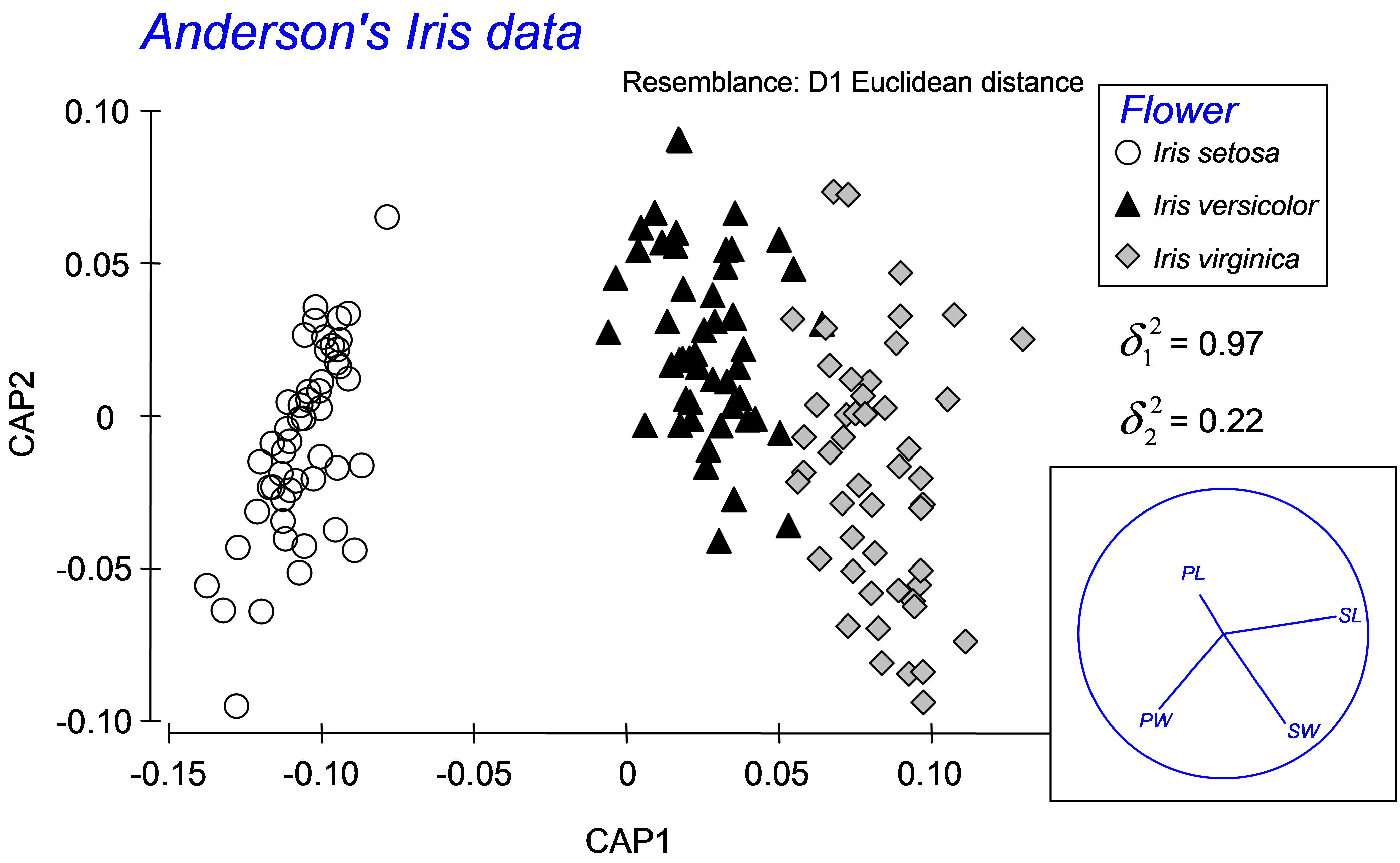Fig. 5.9. Canonical ordination for the discriminant analysis of Anderson’s Iris data.

To proceed with a traditional analysis of the iris data, calculate a Euclidean distance matrix directly from the data and then choose PERMANOVA+ > CAP > (Analyse against •Groups in factor) & (Factor for groups or new samples: Flower) & ($\checkmark$Specify m 4) & (Diagnostics $\checkmark$Do diagnostics > •Chosen m only) & ($\checkmark$Do permutation test > Num. permutations: 9999), then click ‘OK’. We have chosen m = 4 here, because we wish to obtain the classical analysis and there were 4 original variables (PL, PW, SL and SW). The results show that the first squared canonical correlation is very large ($\delta _ 1 ^ 2$ = 0.97) and indeed the first canonical axis does quite a good job of separating the three iris species from one another (Fig. 5.9). The second canonical axis has a much smaller eigenvalue ($\delta _ 2 ^ 2$ = 0.22), and actually there is no clear separation of the groups along this second axis. The role of the original variables can be visualised by superimposing a vector overlay (shown in the inset of Fig. 5.9) using the option Graph > Special > (Vectors •Worksheet variables: iris > Correlation type: Multiple). These vectors show relationships between each of the original individual variables and the CAP axes, taking into account the other three variables in the worksheet (see the section Vector overlays in dbRDA in chapter 4). For these data, petal width and sepal length appear to play fairly important roles in discriminating among the groups. A draftsman plot of the original variables reveals that sepal length and width are highly correlated with one another (r = 0.96) and petal length is also fairly highly correlated with each of these (r > 0.8), so it is not terribly surprising that PL and SW play more minor roles once SL is taken into account.

Diagnostics show that the choice of m = 4 PCO axes includes 100% of the original variation (‘prop.G’ = 1) and that the leave-one-out allocation success was quite high using the canonical model: 93.3% of the samples (140 out of 150) were correctly classified (Fig. 5.10). The most distinct group, which had 100% success under cross-validation, was Iris setosa, whereas the other two species, Iris versicolor and Iris virginica, were a little less distinct from one another, although their allocation success rates were still admirably large (at 92% and 88%, respectively). These results regarding the relative distinctiveness of the groups coincide well with what can be seen in the CAP plot (Fig. 5.9), where the Iris setosa group is indeed easily distinguished and well separated from the other two groups along the first canonical axis.

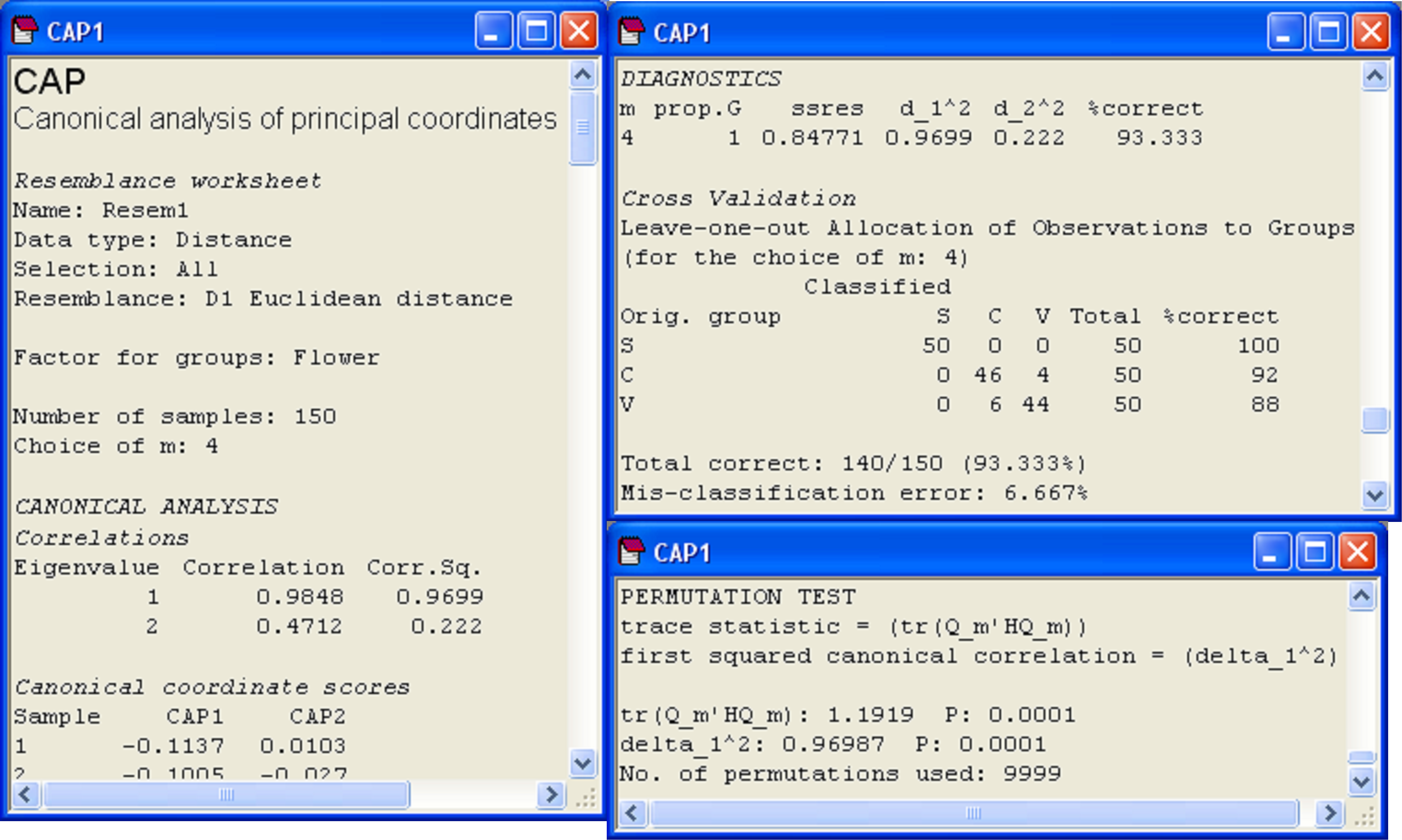Fig. 5.10. Details from the CAP output file for the analysis of Anderson’s iris data.

The results from the permutation tests are shown at the very bottom of the CAP output file (Fig. 5.10). There are two test statistics that are given in the output for the test. The first is a “trace” test statistic. It is the sum of the canonical eigenvalues (i.e., the sum of the squared canonical correlations) or the trace of the matrix Q$^0 _m$′HQ$^0 _m$ (denoted in the output text by ‘tr(Q_m′HQ_m)’). When a CAP analysis is based on Euclidean distance and m = p, then this is equivalent to the traditional MANOVA test statistic known as Pillai’s trace¹⁰⁵. The other test statistic provided in the CAP output is simply the first canonical eigenvalue, which is the first squared canonical correlation, $\delta _ 1 ^ 2$ (denoted in the output text by ‘delta_1^2’). This test statistic is directly related to a statistic called Roy’s greatest root criterion in traditional MANOVA. More specifically, Roy’s criterion is equal to $\delta _ 1 ^ 2$ / (1 – $\delta _ 1 ^ 2$) when $\delta _ 1 ^ 2$ is obtained from a CAP based on Euclidean distances¹⁰⁶ and when m = p. There are other MANOVA test statistics (i.e., Wilks’ lambda, Hotelling-Lawley trace, see Mardia, Kent & Bibby (1979) , Seber (1984) , Rencher (1998) ). Studies show that these different MANOVA test statistics differ in their power to detect different kinds of changes among the group centroids in multivariate space (e.g., Olson (1974) , Olson (1975) , Rencher (1998) ). Olson ( Olson (1974) , Olson (1975) , Olson (1976) ) suggested that Pillai’s trace, although not the most powerful in all situations, did perform well in many cases, and importantly, was quite robust to violations of its assumptions, maintaining type I error rates at nominal levels in the face of non-normality or mild heterogeneity of variance-covariance matrices. It is well known that Roy’s criterion, however, will be the most powerful for detecting changes in means along a single axis in the multivariate space ( Seber (1984) , Rencher (1998) ). Generally, we suggest that the trace criterion will provide the best approach for the widest range of circumstances, and should be used routinely, while the test using the first canonical eigenvalue will focus specifically on changes in centroids along a single dimension, where this is of interest. Of course, the two test statistics will be identical when there is only canonical axis (e.g., two groups).

The permutation test in CAP assumes only exchangeability of the samples under a true null hypothesis of no differences in the positions of the centroids among the groups in multivariate space (for a given chosen value of m). Thus, although the values of the trace statistic and the first squared canonical correlation are directly related to Pillai’s trace and Roy’s criterion, respectively (when Euclidean distance is used), there are no stringent assumptions about the distributions of the variables: tests by permutation provide an exact test of the null hypothesis of no differences in the positions of centroids among groups. Mardia (1971) proposed a permutation test based on Pillai’s trace (e.g., see Seber (1984) ), which would be equivalent to the CAP test on the trace statistic when based on Euclidean distances. Of course, the CAP routine (like all of the routines in PERMANOVA+ for PRIMER) also provides the additional flexibility that any resemblance measure can be used as the basis of the analysis.

---

¹⁰⁵ This equivalence is readily seen by doing a traditional MANOVA using some other statistical package on the Iris data, where the output for Pillai’s trace will be given as 1.1919, the value shown for the trace statistic from the CAP analysis in Fig. 5.10.

¹⁰⁶ See p. 626 of Legendre & Legendre (1998) for more details.