1.20 Fixed vs random factors (Tasmanian meiofauna)
All of the factors considered so far have been fixed, but factors can be either fixed or random. In univariate ANOVA the choice of whether a particular factor is fixed or random has important consequences for the assumptions underlying the model, the expected values of mean squares (thus, the construction of a given F ratio), particularly in more complex designs, the hypothesis tested by the F ratio and, perhaps most importantly, the extent and nature of the inferences. This is also true for PERMANOVA, which follows the analogous univariate ANOVA models in terms of the construction of pseudo-F ratios from expectations of mean squares (EMS).
For a fixed factor, there is a finite set of levels which have been explicitly chosen to represent particular states. These states (the levels) are generally explicit because they have been manipulated (e.g., shade, open and control), because they already exist in nature (e.g., male and female), or because they bear some meaningful relationship to other chosen levels (e.g., high, medium and low). All of the levels of a fixed factor (or at least all of the ones we are effectively interested in) occur in the experiment. So, for a fixed factor, individual levels have a meaning in themselves, and generally, if we were going to repeat the experiment, we would choose the same levels to investigate again (unless we were going to change the hypothesis). The effects of a fixed factor are deemed to be constant values for each nominated state (or level)29. Furthermore, the component of variation attributable to a fixed factor in a given model is considered in terms of the sum of squared fixed effects (divided by the appropriate degrees of freedom). Finally, when we perform the test of the fixed factor, the resulting P-value and any statistical inferences to be drawn from it apply only to those levels and to no others.
For a random factor, however, the particular levels included in the experiment are a random subset from a population of possible levels we could have included (e.g., sites, locations, blocks). We do not consider the individual levels (site 1, site 2, etc.) as representing any particular chosen state. The levels do not have any particular meaning in themselves; we are not interested in comparing, say, site 1 vs site 2, but rather multiple levels of the factor are included to provide us with a measure of the kind of variability that we might expect across the population of possible levels (e.g., among sites). Random factors, unlike fixed factors, actually contribute another source of random variance into the model (in addition to the error variance) and so the effects, rather than being fixed, are instead used to estimate the size of the variance component for that factor. Repeating the experiment would also probably not result in the same levels being chosen again. Importantly, when the F ratio is constructed and the P-value is calculated for a random factor, the statistical inference applies to the variance component for the whole population of possible levels (or effects) that could have been chosen, and not just to the levels included in the experiment.
The difference in the inference space for the fixed versus the random factor is important. For example, if one obtained a P-value less than $\alpha = 0.05$ (the usual convention) for a fixed factor, one might state: “There were significant differences among (say) these three treatments in the structure of their assemblages”. In contrast, for a random factor, one might state: “There was significant variability among sites in the structure of the assemblages.” The fixed factor is more specific and the random factor is more general. Note also that the statement regarding the fixed factor often logically calls for more information, such as pair-wise comparisons between individual levels – which treatments were significantly different from one another and how? Whereas, the second statement does not require anything like this, because the individual levels (sites) are generally not of any further interest in and of themselves (we don’t care whether site 1 differs from site 3, etc.); it is enough to know that significant variability among sites is present. Thus, it is generally not logical to do pair-wise comparisons among levels of a random factor (although PERMANOVA will not prevent you from doing such tests if you insist on doing them)! A logical question to ask, instead, following the discovery of a significant random factor would be: how much of the overall variability is explained by that factor (e.g., sites)? For a random factor, we are therefore more interested to estimate the size of its component of variation and to compare this with other sources of variation in the model, including the residual (see Estimating components of variation).
To clarify these ideas, consider an example of a two-way crossed experimental design used to study the effects of disturbance by soldier crabs on meiofauna at a sandflat in Eaglehawk Neck, Tasmania ( Warwick, Clarke & Gee (1990) ). The N = 16 samples consist of two replicates within each combination of four blocks (areas across the sandflat) and two natural ‘treatments’ (either disturbed or undisturbed by soldier crab burrowing activity). There were p = 56 taxa recorded in the study, consisting of 39 nematode taxa and 17 copepod taxa. We therefore have
-
Factor A: Treatment (fixed with a = 2 levels, disturbed (D) or undisturbed (U) by crabs).
-
Factor B: Block (random with b = 4 levels, labeled simply B1-B4).
The first factor is fixed, because these two treatment levels do have a particular meaning, representing particular states in nature (disturbed or undisturbed) that are of interest to us and that we explicitly wish to compare. In contrast, the second factor in the experiment, Blocks, is random, because we do not have any particular hypotheses concerning the states of, say B1 or B2, but rather, these are included in the experimental design in order to estimate variability across the sandflat at a relevant spatial scale (i.e., among blocks) and to avoid pseudo-replication (sensu Hurlbert (1984) ) in the analysis of treatment effects. A design which has both random and fixed factors is called a mixed model. This particular design (where a fixed factor is crossed with a random one), also allows us to test for generality or consistency in treatment effects across the sandflats.
The data are located in the file tas.pri in the ‘TasMei’ folder of the ‘Examples add-on’ directory. View the factors by choosing Edit>Factors. In order to obtain different symbols for each of the a × b = 2 × 4 = 8 cells in the design, create a new factor whose 8 levels are all combinations of Treatment × Block by choosing ‘Combine’ in the Factors dialog box and then  followed by ‘OK’. Create a resemblance matrix on the basis of Bray-Curtis similarities after square-root transformation. An MDS of these data (as shown in chapter 6 of
Clarke & Warwick (2001)
) shows a clear effect of disturbance on these assemblages, with some variability among the blocks as well (Fig. 1.22).
followed by ‘OK’. Create a resemblance matrix on the basis of Bray-Curtis similarities after square-root transformation. An MDS of these data (as shown in chapter 6 of
Clarke & Warwick (2001)
) shows a clear effect of disturbance on these assemblages, with some variability among the blocks as well (Fig. 1.22).
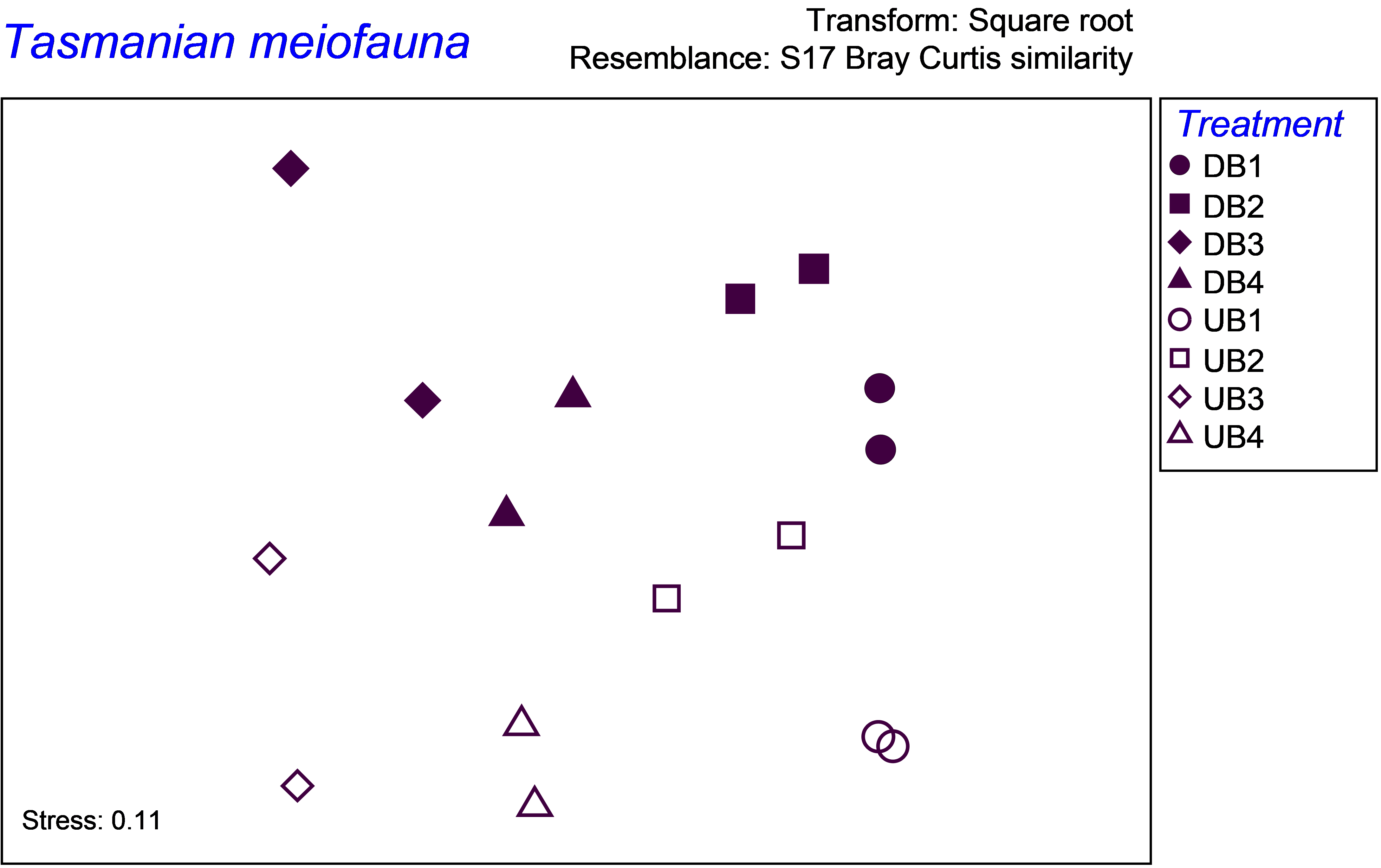 Fig. 1.22. MDS of Tasmanian meiofauna showing variation among the blocks on the x-axis and separation of disturbed from undisturbed communities on the y-axis.
Set up the design file according to the correct experimental design (Fig. 1.23) and rename it as Mixed model, for reference. The next step is to run PERMANOVA on the resemblance matrix according to the mixed model design. Due to the small number of observations per cell, choose (Permutation method ·Unrestricted permutation of raw data) & (Num. permutations: 9999). Save the workspace with the PERMANOVA results as tas.pwk.
The PERMANOVA results show that there is a statistically significant (though borderline) interaction term, indicating that the treatment effects vary from one block to the next (P = 0.044, Fig. 1.23). The MDS plot shows that the direction of the treatment effects appears nevertheless to be fairly consistent across the blocks (at least insofar as this can be discerned using an ordination to represent the higher-dimensional cloud of points), so in this case the significant interaction may be caused by there being slight differences in the sizes of the treatment effects for different blocks.
29 In univariate analysis, the effect for a given group is defined as the deviation of the group mean from the overall mean. Similarly, when using PERMANOVA for multivariate analysis, the effect for a given level is the deviation (distance) of the group’s centroid from the overall centroid in the multivariate space, as defined by the dissimilarity measure chosen.