1.30 Designs that lack replication (Plankton net study)

A topic related to the issue of pooling is the issue of designs that lack replication. Familiar examples are some of the classical experimental designs, primarily from the agricultural literature, such as randomised blocks, split plots or latin squares (e.g. Mead 1988). For these designs the essential issue is that there is no replication of samples within cells, but rather there is only 1 sample per cell. This means that it is not possible to distinguish between variation among samples and variation due to the highest-order (most complex) interaction term. Thus, in order to proceed, the experimenter has either to assume (i) that the highest-order interaction term is zero, or (ii) that the so-called “residual” mean square in the model actually has expectation V(Res) + V(highest-order interaction). Note that, for the latter assumption to work, at least one of the factors involved in the highest-order interaction has to be random. See Gates (1995) and chapter 10 of Quinn & Keough (2002) for further discussion of these issues.

From a practical perspective, for PERMANOVA to proceed with the analysis (regardless of which of the above two perspectives one chooses to take), the highest-order interaction term needs to be excluded from the analysis (see the section Pooling or excluded terms, above). This can either be done manually, or if the PERMANOVA routine detects that there is no within-cell replication, then it will issue a warning. If you choose to proceed by clicking ‘OK’, it will automatically exclude the highest-order interaction term from the model. If you receive this warning and you know that you do have within-cell replication, then there is a very good chance that you have mis-labeled your factor levels somehow³⁵.

An example of a two-way crossed design without replication is provided in a study by Winsor & Clarke (1940) Winsor & Clarke (1940) to investigate the catch of various groups of plankton by two nets hauled horizontally, with one net being 2 metres below the other. Ten hauls were made with the pair of nets at depths of 29 and 31 meters, respectively. The experimental design is:

Factor A:	Position (fixed with a = 2 levels, either upper (U) or lower (L) depths).
Factor B:	Haul (random with b = 10 levels, labeled simply 1-10).

There is only 1 value per combination of treatments, with no replication, so N = a × b = 20. This is effectively a randomised block design, where the hauls are “blocks”. The variables recorded correspond to five different groups of plankton. Standard deviations in the various groups were roughly proportional to the means, so data were transformed and are provided as logarithms of the catch numbers for each of the plankton groups. These data are located in the plank.pri file in the ‘Plankton’ folder of the ‘Examples add-on’ directory, and were provided by Snedecor (1946) .

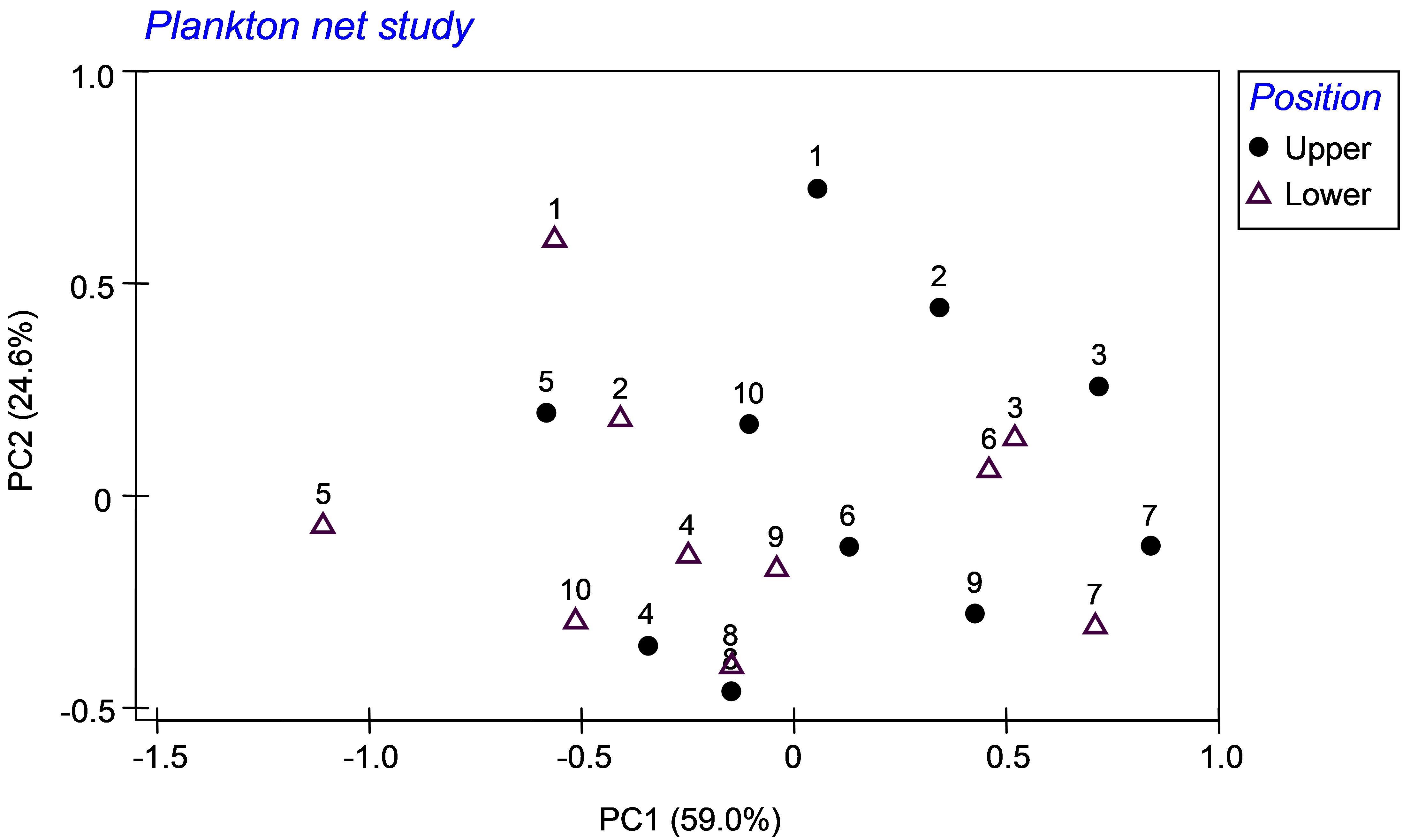
Fig. 1.33. PCA of the study of plankton from ten hauls (numbered) at either 29 m depth (upper) or 31 m depth (lower).

Examination of the data (already log-transformed) reveals no zeros and that their distributions are fairly even, with no extreme values or outliers³⁶. The variables are also on similar scales and are measured in the same units; therefore, an analysis based directly on Euclidean distances would be reasonable here – prior normalisation is not necessary. For data like these, an appropriate ordination method is principal components analysis (PCA)³⁷. The first two principal components explained 83.6% of the total variance in the five variables (Fig. 1.33). Variability among the hauls is apparent in the diagram, but a clear difference in the plankton numbers due to the position of the nets (upper versus lower), if any, is not obvious.

The PERMANOVA analysis of these data on the basis of a Euclidean distance matrix has detected significant variability among the hauls, but also has detected a significant effect of the position of the net (Fig. 1.34). Notice that the output has identified the excluded term: ‘PositionxHaul’, as an important reminder that the analysis without replication is not without an additional necessary assumption in this regard.

It might seem surprising that the analysis has detected any effect of ‘Position’ at all, given the pattern seen in the PCA (Fig. 1.33). Looks can be deceiving, however. Close inspection of the plot reveals that, within almost all of the individual hauls (i.e., 1, 2, 3, 5, 7, 9, 10), the symbol for the ‘upper’ group lies to the right of the symbol for the ‘lower’ group. Only hauls 4, 6 and 8 do not conform to this pattern. We can perhaps understand the nature of this overall effect of Position by examining the averages for the ‘upper’ and ‘lower’ nets for each of the variables across all of the hauls. With the Plankton worksheet highlighted, select Tools > Average > (Samples •Averages for factor: Position) & (Variables •No averaging). The resulting worksheet shows that the average log(abundance) for all five of the plankton variables was larger for the nets towed at the shallower depth (the ‘upper’ nets) (Fig. 1.34).

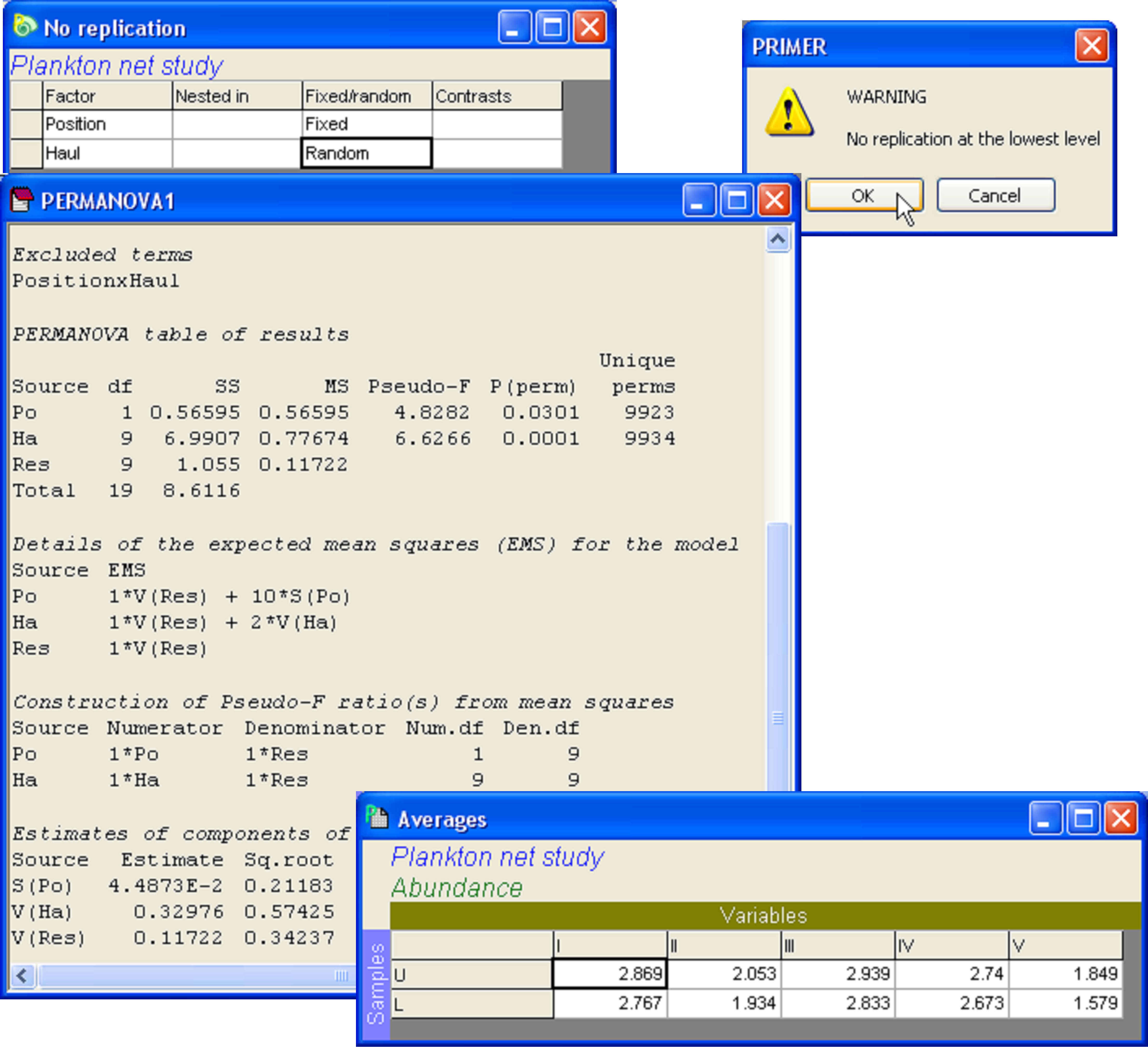
Fig. 1.34. Design file and PERMANOVA analysis for the two-way study that lacks replication within cells. The interaction term is, by necessity, excluded from the analysis, as it is already confounded with the residual variance. Also shown are the averages per depth for each of the 5 variables in the plankton study.

Another important point here is to recognise that, had we treated the above design as if the hauls were the replicates, and ignored the variation among hauls, then we would not have detected any effect of position at all. You can check this fact by running PERMANOVA on the data using a one-way design with the factor ‘Position’ only (the result is non-significant, with P > 0.25). Thus, despite the fact that there is a consistent shift in the plankton assemblage between the upper and lower nets within each haul, the variation from haul to haul would have masked this entirely and we would have failed to detect it (as we at first did when contemplating the PCA plot), if we had not included the factor ‘Haul’ in our analysis. The advantages of “blocking” to achieve greater power to detect treatment effects have been known for a very long time (e.g., Fisher (1935) , Snedecor (1946) , Mead (1988) ), but this example shows that the phenomenon can occur equally strikingly in the analysis of multivariate data.

The analysis of some other designs that lack replication have other issues, on top of the one already noted regarding the highest-order interaction being inextricably confounded with the residual. For example, the experimental design known as the latin square consists of a random allocation of t treatments to a t × t matrix of sample units, with the added constraint that there be one of every treatment in every row and one of every treatment in every column of this array. The usual model fitted to such a design partitions the sum of squares according to the following sources: rows (R), columns (C) and treatments (T). None of the potential interaction terms (R×C, R×T, C×T, R×C×T) are traditionally included in these models, because none of them can be readily unconfounded from the residual. PERMANOVA does not have separate subroutines for treating these kinds of special designs, but will not give sensible results³⁸ unless the terms which cannot be estimated are first removed from the model. For these more complex designs lacking replication, it is up to the user to know if such interactions need to be excluded, to understand the consequences of the assumptions underlying these models if they are to be used, and to exclude the relevant terms manually, using the ‘Terms…’ button in the PERMANOVA dialog.

---

³⁵ For example, you may have given the levels of factor B the names b1, b2, b3 within the first level of factor A, but then called them B1, B2, B3 within the second level of factor A, and PRIMER will not interpret these names as being the same.

³⁶ PRIMER’s Analyse>Draftsman plot routine is very useful for visually examining the distributions and joint distributions of variables in a worksheet.

³⁷ For more details regarding this method and its implementation in PRIMER, see chapter 4 of Clarke & Warwick (2001) and chapter 10 in Clarke & Gorley (2006) .

³⁸ (or, at least, not the results that are traditionally provided for such designs).