4.13 dbRDA plot for Ekofisk
Let us examine the constrained dbRDA ordination for the parsimonious model obtained earlier using DISTLM on the Ekofisk data. The parsimonious model we had settled on included three predictor variables: (Distance)^(0.25), sqr(Ba) and sqr(Sr). Go to the ekevt worksheet, highlight and then select these three variables by choosing Select > Highlighted. Now return to the resemblance matrix based on the macrofaunal data and choose PERMANOVA+ > dbRDA > (Predictor variable worksheet: ekevt) & (Max. no. of dbRDA axes: 3) & ($\checkmark$Plot results). The resulting pattern among the samples (Fig. 4.16) suggests that there are effectively two gradients (forming sort of an upside-down “V” shape) in the community structure of the macrofauna that can be modeled by these environmental variables. The first largely distinguishes among groups A, B, C and D and is (not surprisingly) driven largely by distance from the oil platform, as well as the concentrations of Ba in the sediments. The second gradient identifies variability among the sites within group D that are close to the oil platform (< 250 m). These differences are apparently mostly driven by differences in the concentrations of Sr in the sediments. We shouldn’t forget, however, that sqr(Sr) had a very strong relationship (r = 0.92) with log(THC), so the modeled variation in community structure among these samples near the platform could just as easily be due to variation in total hydrocarbons as to strontium concentrations (or to the combined effects of both, or to some other unmeasured variables)91.
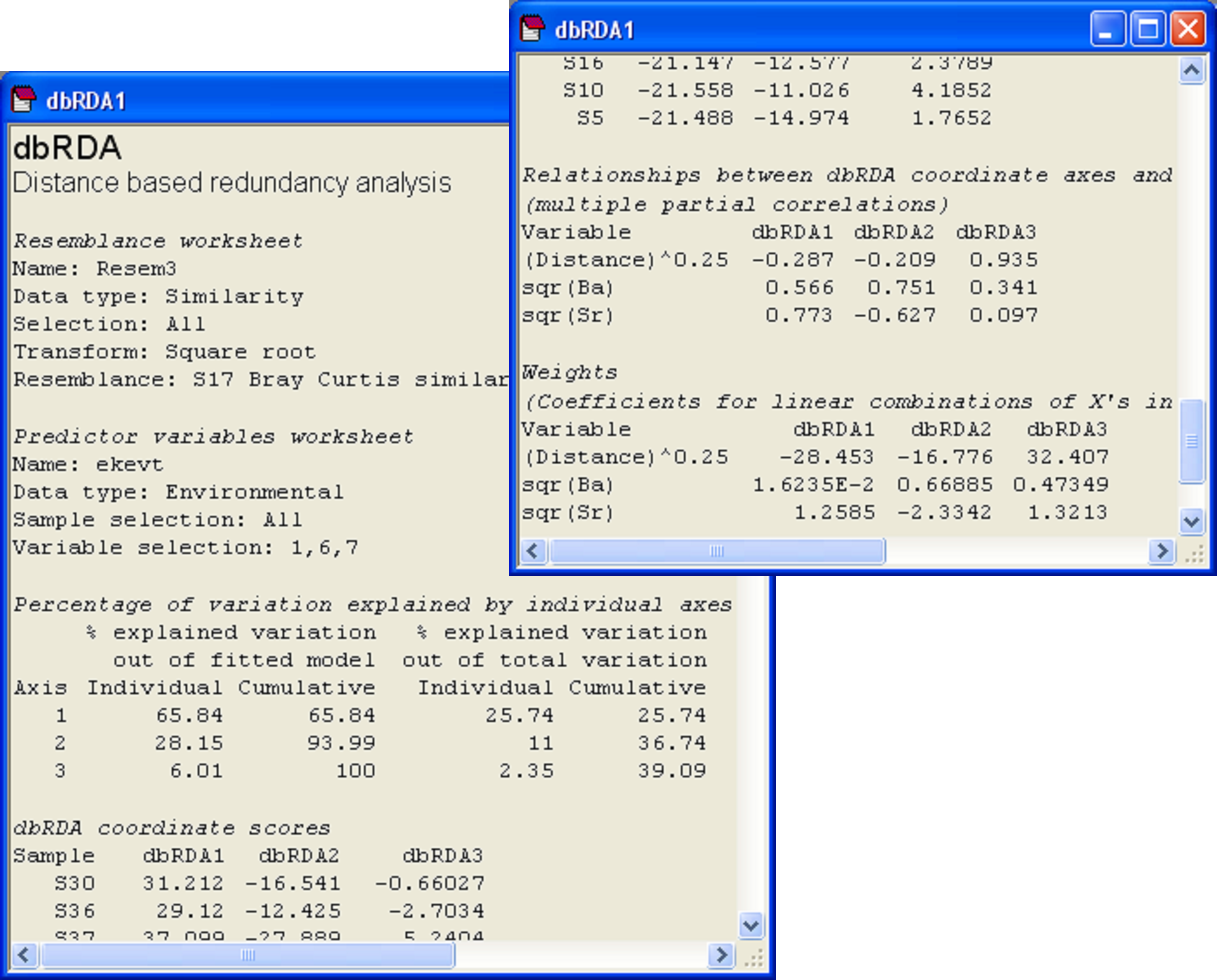
Fig. 4.17. Output file from dbRDA of the Ekofisk macrofauna vs three environmental variables.
Other output provided from running the dbRDA routine shows more information about the dbRDA axes (Fig. 4.17). First, we are given information that will help to assess the adequacy of the ordination plot. The first two columns in the section entitled ‘Percentage of variation explained by individual axes’ relate to the percentage explained out of the fitted model (i.e., out of tr(HGH) or SS$_ \text{Regression} $). The next two columns in this section relate to the percentage explained out of the total variation in the resemblance matrix (i.e., out of tr(G) or SS$_ \text{Total} $). In the present case, the first two dbRDA axes explain 94.0% of the fitted variation, and this is about 36.7% of the total variation in the resemblance matrix. So, we can rest assured that these two dbRDA axes are capturing pretty much everything we should wish to know about the fitted model, although there is sill quite a lot of residual variation in the original data matrix which is not captured in this diagram. Note that there are three dbRDA axes as s = min( q, (N – 1) ) = min( 3, 38 ) = 3. All of the dbRDA axes together explain 100% of the fitted variation. Taken together, they also explain 39.1% of the total variation. This is equal to 100 × R$^2$ from the DISTLM model for these three variables (Fig. 4.13).
Another way to check the overall utility and adequacy of the model as it is shown in the constrained dbRDA plot is to compare it with an unconstrained PCO plot of the same data. If the patterns of sample points in the two plots are similar, then this indicates that the dbRDA (and by implication, the model) is doing a good job of finding and explaining the most salient patterns of variation across the data cloud as a whole. If, on the other hand, these two plots are quite different, then, although it does not mean the model is useless, it does indicate that there are likely to be some other structuring forces out there which were not measured or included in the model. The PCO plot of the Ekofisk data shows a remarkably similar pattern to the dbRDA plot (Fig. 4.18), indicating that this three-variable model is indeed capturing the most salient overall patterns of variability. Although there is still quite a lot of unexplained variation (even the first two PCO axes explain only 43.1% of the total), these are the axes of greatest variation through the data cloud defined by the resemblance measure chosen and thus the environmental drivers used in the model (and variables correlated with them) are very likely to be the most important drivers of differences in macrofaunal community structure among these samples.
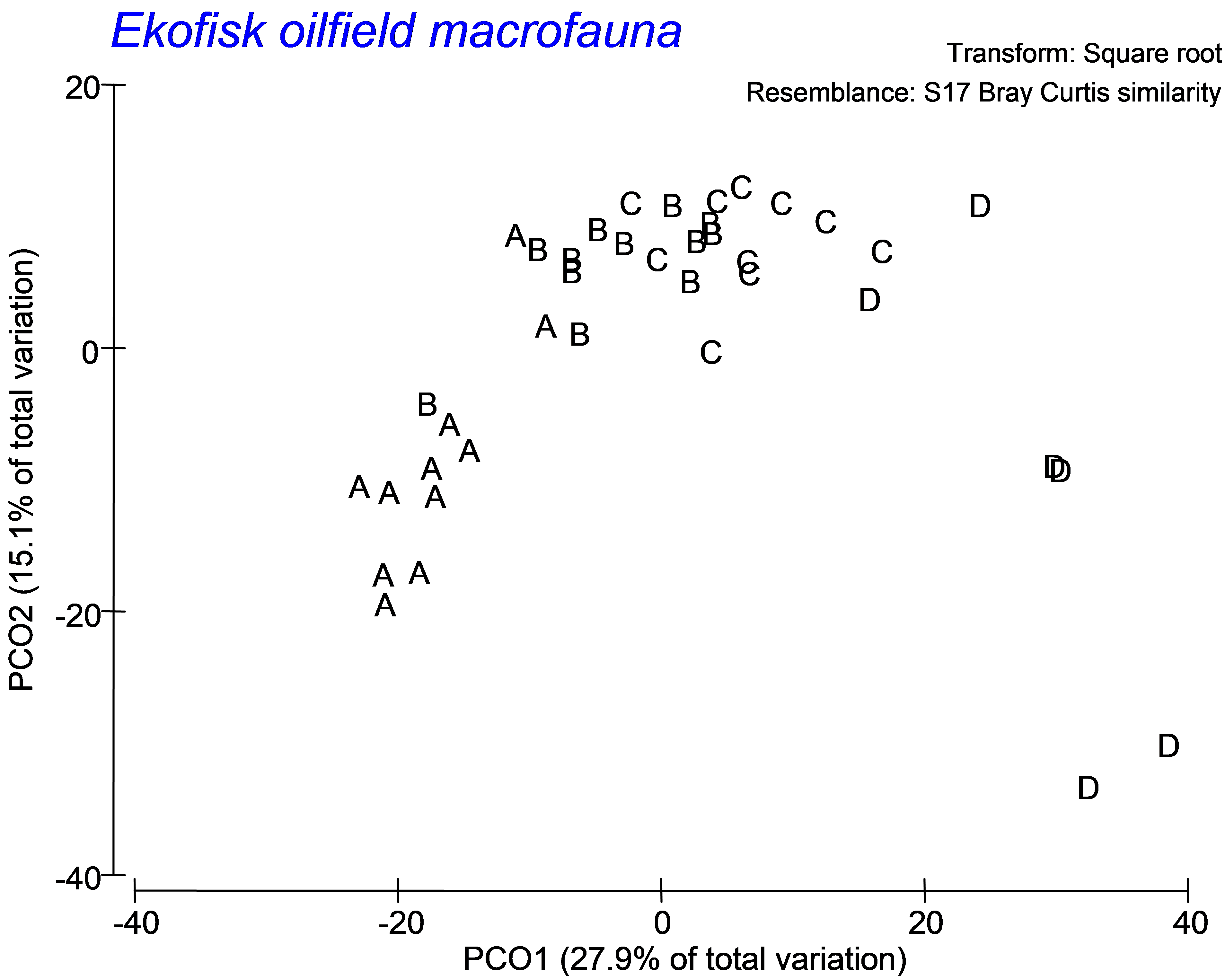 Fig. 4.18. PCO of the Ekofisk macrofauna.
The next portion of the output file provides the dbRDA coordinate scores (Fig. 4.17). These are the positions of the samples along the dbRDA axes and they can also be output into a separate worksheet by ticking the ($\checkmark$Scores to worksheet) option in the dbRDA dialog. Next, the output file provides information regarding the vector overlay positions of each variable along each axis (Fig. 4.17). Specifically, under the heading ‘Relationships between dbRDA coordinate axes and orthonormal X variables’, are given the values of the multiple partial correlations; these are the values that are plotted in the default dbRDA vector overlay.
The last portion of the output from dbRDA shows the relative importance of each X variable in the formation of the dbRDA axes (Fig. 4.17). These are entitled ‘Weights’ and subtitled ‘(Coefficients for linear combinations of X's in the formation of dbRDA coordinates)’. Recall that the dbRDA axes are linear combinations of the fitted values and that these, in turn, are linear combinations of the original X variables. Thus, we can obtain the direct conditional relationships of individual X variables in the formation of each dbRDA axis by multiplying these two sets of linear combinations together. The resulting weights given here are identical to the standardised partial regression coefficients that would be obtained by regressing each of the dbRDA axes scores (Z) directly onto the matrix of normalised explanatory variables X92.
91 Quite similar roles for Ba and THC as those described here were outlined for this data set by Clarke & Gorley (2006) (p. 84, chapter 7) from examining bubble plots of these environmental variables on the species MDS plot, although no formal modeling of these relationships was done in that purely non-parametric setting.
92 If a Euclidean distance matrix was used as the basis of the dbRDA analysis, these weights correspond precisely to the matrix called C in equation 11.14 on p. 585 of Legendre & Legendre (1998) .