3.5 Negative eigenvalues

The sharp-sighted will have noticed a conundrum in the output given for the Victorian avifauna shown in Fig. 3.2. The values for the percentage variation explained for PCO axes 10 through 15 are negative! How can this be? Variance, in the usual sense, is always positive, so this seems very strange indeed! It turns out that if the resemblance measure used is not embeddable in Euclidean space, then some of the eigenvalues will be negative, resulting in (apparently) negative explained variation. How does this happen and how can it be interpreted?

Negative eigenvalues can occur when the resemblance measure used does not fulfill the four mathematical properties required for it to be classified as a metric distance measure. These are:

1. The minimum distance is zero: if point A and point B are identical, then $d _ {AB} = 0$.
2. All distances are non-negative: if point A and point B are not identical, then $d _ {AB} > 0$.
3. Symmetry: the distance from A to B is equal to the distance from B to A: $d _ {AB} = d _ {BA}$.
4. The triangle inequality: $d _ {AB} \le ( $d _ {AC} + $d _ {BC} )$.

Almost all measures worth using will fulfill at least the first three of these properties. A dissimilarity measure which fulfills the first three of the above properties, but not the fourth, is called semi-metric. Most of the resemblance measures of greatest interest to ecologists are either semi-metric (such as Bray-Curtis) or, although metric, are not necessarily embeddable in Euclidean space (such as Jaccard or Manhattan) and so negative eigenvalues can still be produced by the PCO⁶⁶.

The fourth property, known as the triangle inequality states that the distance between two points (A and B, say) is equal to or smaller than the distance from A to B via some other point (C, say). How does violation of the triangle inequality produce negative eigenvalues? Perhaps the best way to tackle this question is to step through an example.

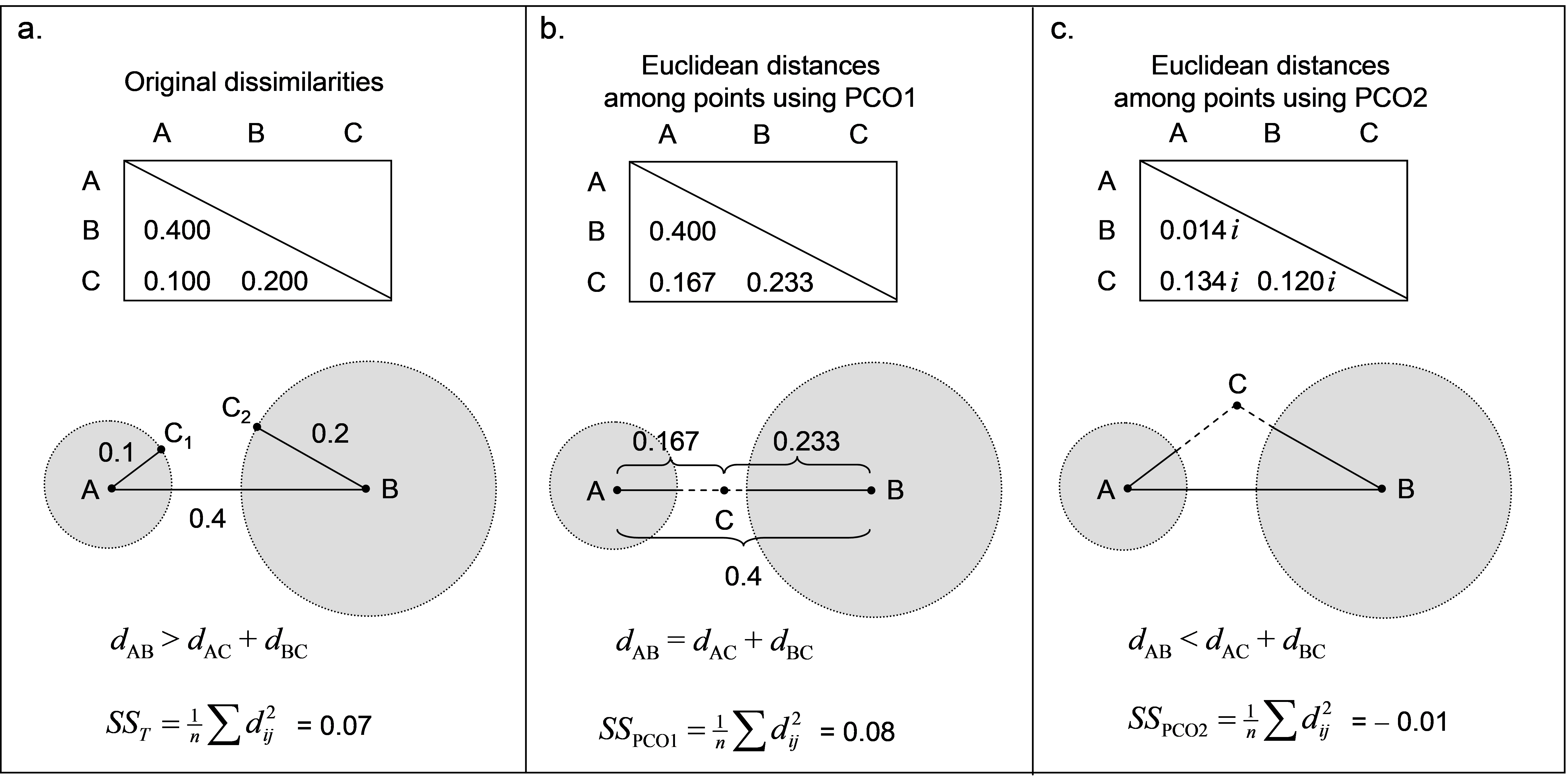Fig. 3.4. Demonstration of violation of the triangle inequality and how PCO generates a Euclidean solution in two dimensions; the second dimension is imaginary.

Consider a resemblance measure calculated among three points: A, B and C, which produces the dissimilarity matrix shown in Fig. 3.4a. Here, the triangle inequality is clearly violated. Consequently, there is no way to place these three points into Euclidean space in two real dimensions in such a manner which preserves all three original dissimilarities. Point C should lie at a distance of 0.1 from point A (i.e., it may lie at any position along the circumference of a circle of radius 0.1 whose centre is at point A, such as C$_ 1$). However, point C should also lie at a distance of 0.2 from point B (such as at point C$_ 2$). Clearly, point C cannot fulfil both of these criteria simultaneously – it cannot be in two places at once! Well, we have to put point C somewhere in order to draw this configuration in Euclidean space (i.e., on the page) at all. Suppose point C is given a position along a single dimension between points A and B, as shown in Fig. 3.4b. This could be anywhere, perhaps, along the straight-line continuum from A to B, but it would make sense for it to lie somewhere in the “gap” between the two circles. If we had done a PCO of the original dissimilarity matrix, the position for point C shown in Fig. 3.4b is precisely that which is given for it along the first PCO axis.

Clearly, in order to draw this ordination (in one dimension), we have had to “stretch” the distances from A to C and from B to C, just so that C could be represented as a single point in the diagram. A consequence of this is that the total variation (the sum of squared inter-point distances divided by the number of points, see Figs. 1.3 and 1.4 in chapter 1) is inflated. That is, the original total sum of squares was $SS _ T$ = 0.07 (Fig. 3.4a), and now, even using only one dimension, the total sum of squares is actually larger than this ($SS _ {PCO1}$ = 0.08, Fig. 3.4b). We can remove this “extra” variance, introduced by placing the points from a semi-metric system into Euclidean space, by introducing one or more imaginary axes. Distances along an imaginary axis can be treated effectively in the same manner as those along real axes, except they need to be multiplied by the constant $ i = \sqrt{-1}$. Consequently, squared values of distances along an imaginary axis are multiplied by $i ^ 2 = -1$, and, therefore, are simply negative. In our example, the distances among the three points obtained along the second PCO axis (which is imaginary) are shown in Fig. 3.4c. In practice, the configuration output treats the second axis like any other axis (so that it can be drawn), but we need to keep in mind that this second axis (theoretically and algebraically) is actually defined only in imaginary space⁶⁷. The total sum of squares along this second axis alone is $SS _ {PCO2} = – 0.01$, and so the variance occurring along this imaginary axis is negative. Despite this, we can see in this example that $SS _ T = SS_ {PCO1} + SS_ {PCO2}$. It is true in this example, and it is true in general, that the sum of the individual SS for each of the PCO’s will add up to the total SS from the original dissimilarities provided we take due care when combining real and imaginary axes – the SS of the latter contribute negatively. In this example, there is one positive and one negative eigenvalue, corresponding to PCO1 and PCO2, respectively. The sum of these two eigenvalues, retaining their sign, is equal to the total variance.

Returning now to the Victorian avifauna, we can plot the percentage of the variation explained by each of the PCO axes, as given in the output in Fig. 3.2. This is known as a scree plot (Fig. 3.5), and it provides a visual diagnostic regarding the number of axes that capture the majority of variation for this system. For this example, there are a series of positive eigenvalues which are progressively smaller in size, followed by a series of negative eigenvalues (Fig. 3.5). We can also plot these percentages cumulatively (Fig. 3.5) and see that the percentage of explained variation goes up past 100% when we get to PCO axis 5. The first 9 PCO axes together actually explain ~106% of the original variation (Fig. 3.2). Once again, the reason for this is that the analysis has had to “make do” and “stretch” some of the original distances (for which the triangle inequality does not hold) in order to represent these points on real Euclidean axes. Then, with the addition of subsequent PCO axes (10 through 15) corresponding to negative eigenvalues (imaginary Euclidean axes), this is brought back down to precisely 100% of the original variation based on adjusted Bray-Curtis resemblances.

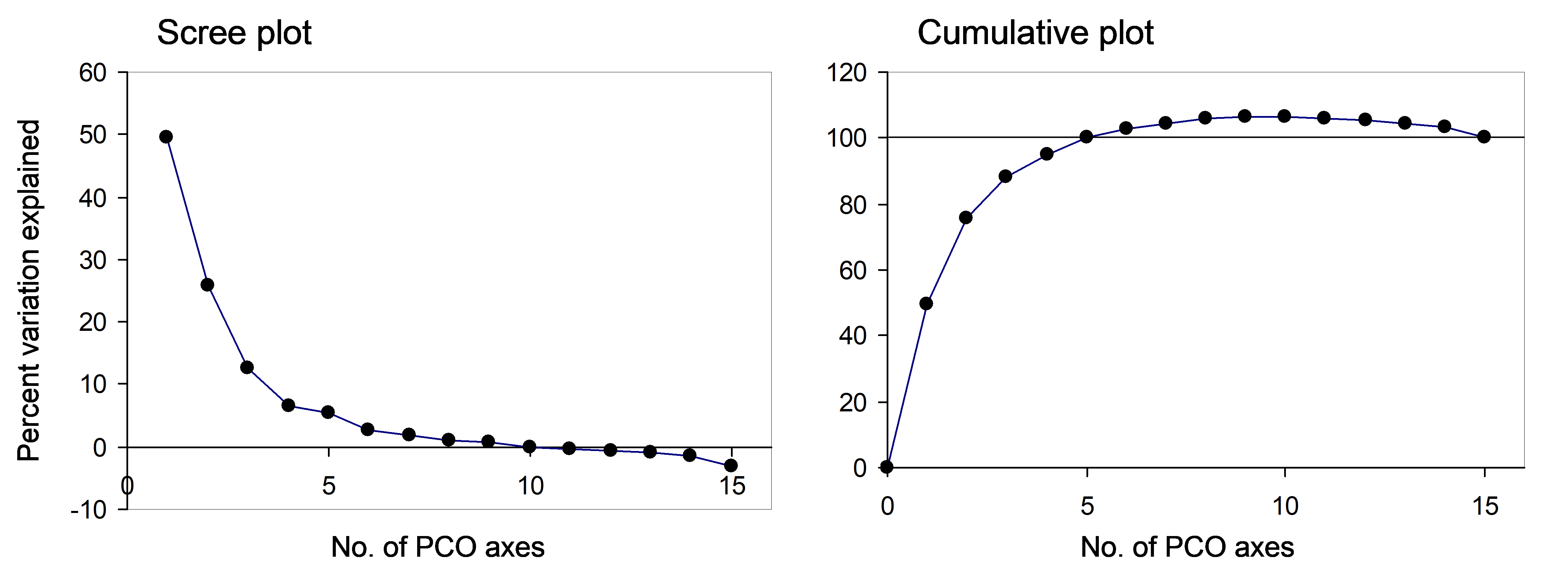Fig. 3.5. Scree plot and cumulative scree plot for the PCO of the Victorian avifauna data.

For purposes of ordination, our interest will be in plotting and visualising patterns using just the first two or three axes. Generally, these first few axes will correspond to large positive eigenvalues, the axes corresponding to negative eigenvalues will be negligible (i.e., in the “tail” of the scree plot) and need not be of any concern Sibson (1979) , Gower (1987) ). However, if:

• the first two or three PCO axes together explain > 100% of the variation,
• any of the plotted PCO axes are associated with a negative eigenvalue (i.e. corresponding to an imaginary axis), or
• the largest negative eigenvalue in the system as a whole is larger (in absolute value) than the smallest positive eigenvalue associated with the PCO axes in the plot (, as cited by Legendre & Legendre (1998) ,

then interpreting the plot will be problematic. In any of these cases, one would be dealing with a resemblance matrix that rather seriously violates the triangle inequality. This can occur if the resemblance measure being used is inappropriate for the type of data, if there are a lot of repeated values in the resemblance matrix or if the resemblances are ranked prior to analysis. With the PCO routine, as with PERMANOVA or PERMDISP, it makes sense to carefully consider the meaning of the resemblance measure used in the context of the data to be analysed and the questions of interest.

Perhaps not surprisingly, previous workers have been troubled by the presence of negative eigenvalues from PCO analyses and how they should be interpreted (e.g., see pp. 432-438 in Legendre & Legendre (1998) ). One possibility is to “correct” for negative eigenvalues by adding a constant to all of the dissimilarities ( Cailliez (1983) ) or to all of their squares ( Lingoes (1971) ). Clearly, these correction methods inflate the total variation (e.g., Legendre & Anderson (1999) ) and are not actually necessary ( McArdle & Anderson (2001) ). Caillez & Pagès 1976 also suggested correcting the percentage of the variation among N points explained by (say) the first m PCO axes from what is used above, i.e.: $$ 100 \times \frac{\sum _ {i=1} ^ m \lambda _i }{\sum _ {i=1} ^ N \lambda _i } \tag{3.1} $$ to: $$ 100 \times \frac{\sum _ {i=1} ^ m \lambda _i +m |\lambda _N ^{-} | }{\sum _ {i=1} ^ N \lambda _i (N -1)|\lambda _ N ^ {-} |} \tag{3.2} $$ where $ |\lambda _ N ^ {-} | $ is the absolute value of the largest negative eigenvalue (see p. 438 in Legendre & Legendre (1998) ). Although it was suggested that (3.2) would provide a better measure of the quality of the ordination in the presence of negative eigenvalues, this is not entirely clear. The approach in (3.2), like the proposed correction methods, inflates the total variation. Alternatively, Gower (1987) has indicated that the adequacy of the ordination can be assessed by calculating percentages using the squares of the eigenvalues, when negative eigenvalues are present. In the PCO routine of the PERMANOVA+ package, we chose simply to retain the former calculation (3.1) in the output, so that the user may examine the complete original diagnostic information regarding the percentage of variation explained by each of the real and imaginary axes, individually and cumulatively (e.g., Figs. 3.2 and 3.5).

An important take-home message is that the PCO axes together do explain 100% of the variation in the original dissimilarity matrix (Fig. 3.4), provided we are careful to retain the signs of the eigenvalues and to treat those axes associated with negative eigenvalues as imaginary. The PCO axes therefore (when taken together) provide a full Euclidean representation of the dissimilarity matrix, albeit requiring both real and complex (imaginary) axes for some (semi-metric) dissimilarity measures. As a consequence of this property, note also that the original dissimilarity between any two samples can be obtained from the PCO axes. More particularly, the square root of the sum of the squared distances between two points along the PCO axes⁶⁸ is equal to the original dissimilarity for those two points. For example, consider the Euclidean distance between points A and C in Fig. 3.4 that would be obtained using the PCO axes alone: $$ d _ {AC} = \sqrt{ \left( d _ {AC} ^ {PCO1} \right) ^ 2 + \left( d _ {AC} ^ {PCO2} \right) ^ 2 } = \sqrt{ \left( 0.167 \right) ^ 2 + \left( 0.134 i \right) ^ 2}. $$ As $i^2 = -1$, this gives $$ d _ {AC} = \sqrt{ \left( 0.167 \right) ^ 2 - \left( 0.134 \right) ^ 2} = 0.100$$ which is the original dissimilarity between points A and C in Fig. 3.4a. In other words, we can re-create the original dissimilarities by calculating Euclidean distances on the PCO scores ( Gower (1966) ). In order to get this exactly right, however, we have to use all of the PCO axes and we have to treat the imaginary axes correctly and separately under the square root sign (e.g., McArdle & Anderson (2001) ).

---

⁶⁶ For a review of the mathematical properties of many commonly used measures, see Gower & Legendre (1986) and chapter 7 of Legendre & Legendre (1998) .

⁶⁷ Indeed, for any other purposes apart from attempts to physically draw a configuration, PRIMER and the PERMANOVA+ add-on will indeed treat such axes, algebraically, as imaginary, and so maintain the correct sign of the associated eigenvalue.

⁶⁸ (i.e., the Euclidean distance between two points calculated from the PCO scores)