1.2 Partitioning
We shall begin by considering the balanced one-way (single factor) ANOVA experimental design. A factor is defined as a categorical variable that identifies several groups, treatments or levels which we wish to compare. Imagine that we have one factor with a groups (or levels) and n observations (samples5) per group for a total of N = a × n samples. For each sample, we have recorded the values for each of p different variables. Recall that in univariate analysis of variance, the total sum of squares ($SS _ T$, the sum of squared deviations of observations from the overall mean) is partitioned into two parts that are meaningful for testing hypotheses about group differences: the within-group (or residual) sum of squares ($SS _ {Res}$, the sum of squared deviations of observations from their own group mean) and the among-group sum of squares ($SS _ A$, the sum of squared deviations of group means from the overall mean). A directly analogous partitioning is done in multivariate space by PERMANOVA.
PERMANOVA may be thought of as a method that takes a geometrical approach to MANOVA ( Edgington (1995) ). Let each of the p variables be a dimension, and each of the N samples be represented by points in the p-dimensional space according to the values they take for each variable along each dimension. Now, the simplest of all multivariate systems has only p = 2 variables. It is good to consider this situation, because it is easy to draw just 2 dimensions! Now, imagine that there were n = 10 replicate samples in each of a = 3 groups, as shown in Fig. 1.1.
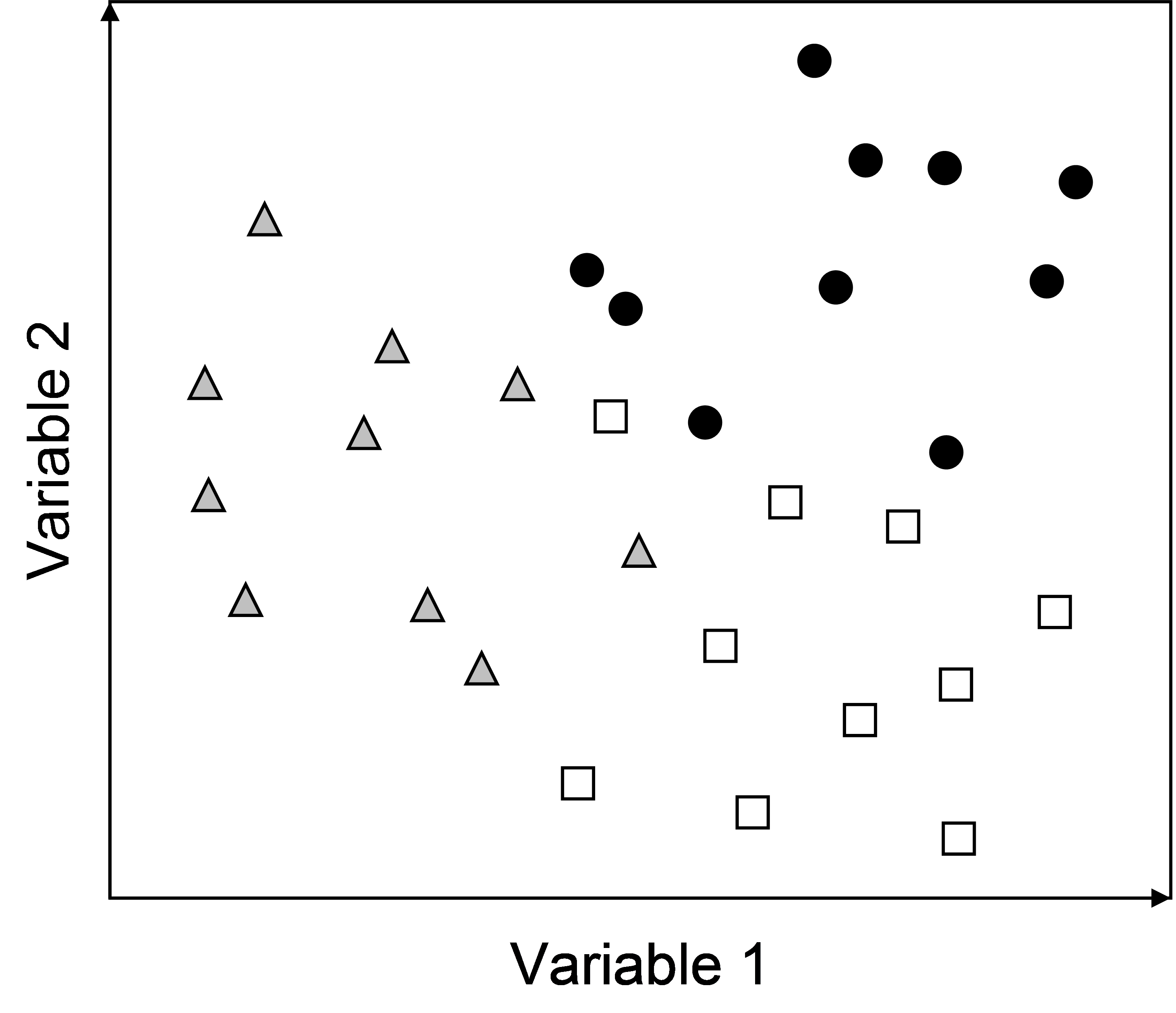 Fig. 1.1. Plot of a hypothetical data set with p = 2 variables (dimensions) and n = 10 replicate samples in each of a = 3 groups. The three groups are identified by different symbols in the plot.
The whole set of N = 30 samples taken together create a data cloud which is centred on a point called the overall centroid. For a Euclidean system, this is obtained as the arithmetic average for each of the (in this case 2) variables. Similarly, each of the groups also has its own group centroid, located in the centre of each of the clouds of points identified for each group.
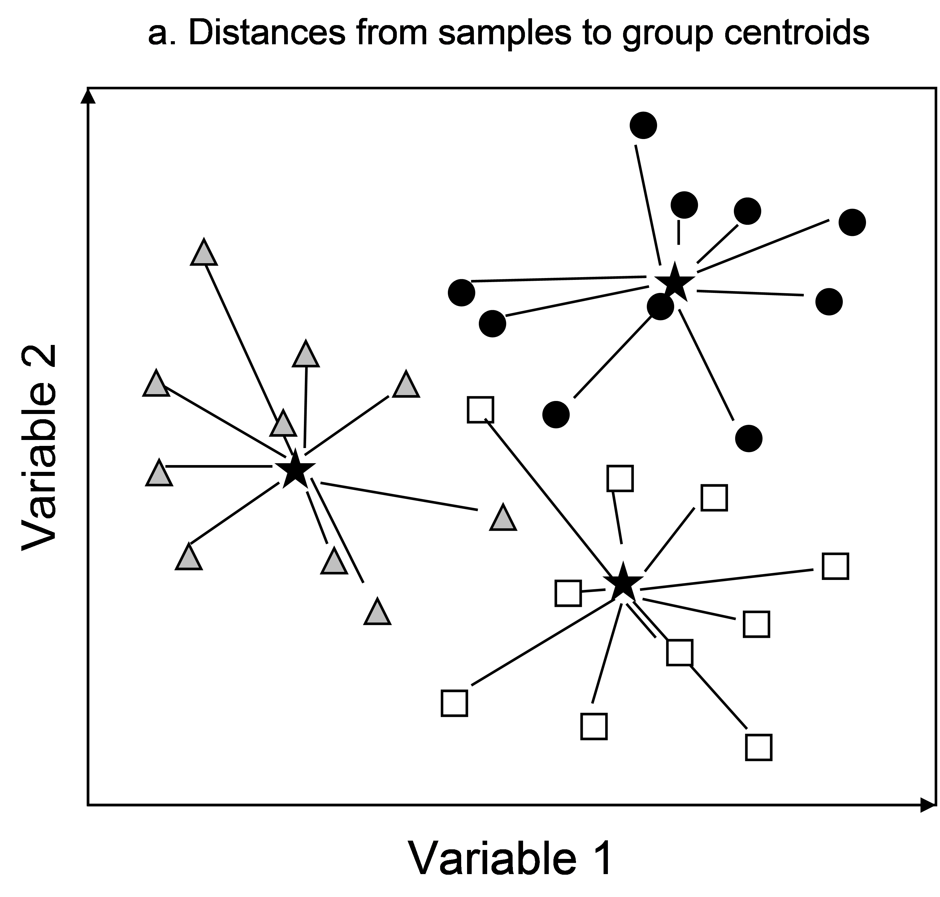
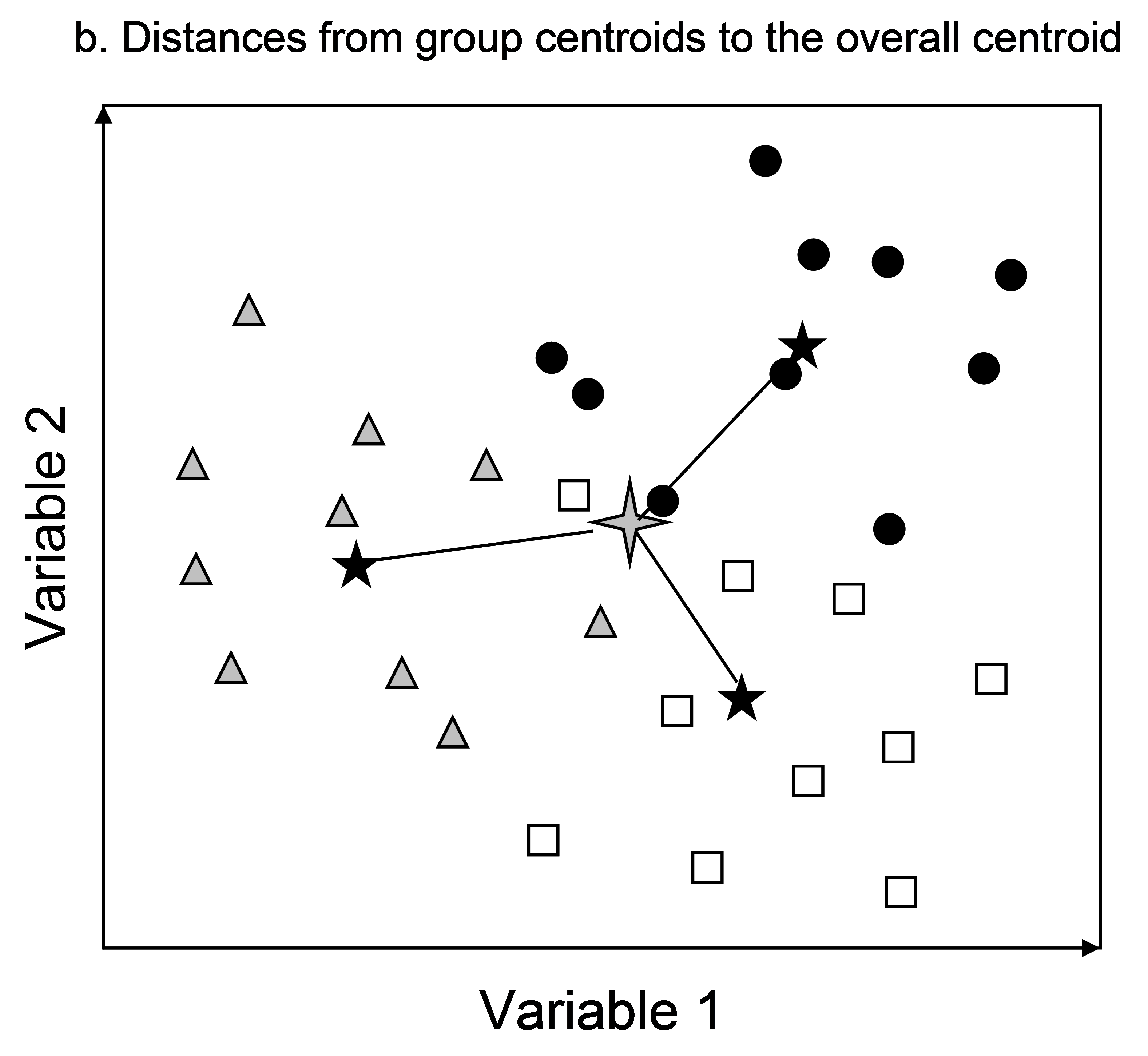 Fig. 1.2. Plots of the hypothetical data set from Fig. 1.1 showing the geometric partitioning.
Just as in univariate ANOVA, we can consider the distance of any given point (sample) from the overall centroid in this space as being made up of two parts: the distance from the point to its group centroid (Fig. 1.2a) plus the distance from the group centroid to the overall centroid (Fig. 1.2b). This is the essence of the geometric approach to MANOVA in Euclidean space. We can calculate the sums of squares as:
$SS _ T$ = the sum of squared distances from the samples to the overall centroid,
$SS _ {Res}$ = the sum of squared distances from the samples to their own group centroid, and
$SS _ A$ = the sum of squared distances from the group centroids to the overall centroid.
The well-known univariate ANOVA identity: $SS _T = SS _ {Res} + SS _ A$ also holds for this geometric conception of MANOVA in Euclidean space. Verdonschot & ter Braak (1994) and Legendre & Anderson (1999) also remark on how these sums of squares are equal to the sum of the individual univariate sums of squares for each of the separate variables if Euclidean distance is used.
5 The word sample will be used throughout this manual in the manner that ecologists, and not statisticians, have come to understand the word. A sample shall mean a single unit used for sampling, such as a core, a transect, or a quadrat. This is consistent with the use of this word in PRIMER.