1.27 Nested design (Holdfast invertebrates)

We have seen how a crossed design is identifiable by virtue of every level of one factor being present in every level of the other factor, and vice versa (e.g., Fig. 1.14). We can contrast this situation with a nested design. A factor is nested within another (upper-level) factor if its levels take on different identities within each level of that upper-level factor.

For example, consider a study by Anderson, Diebel, Blom et al. (2005) of the spatial variability in assemblages of invertebrates colonising holdfasts³² of the kelp Ecklonia radiata in northeastern New Zealand. An hierarchical sampling design was used (Fig. 1.26). Divers collected $n = 5$ individual holdfasts (separated by metres) within each of 2 areas (separated by tens of metres) within each of 2 sites (separated by hundreds of metres to kilometers), within each of 4 locations (separated by hundreds of kilometers) along the coast. The design was balanced and fully nested with three factors:

Factor A:	Locations (random with a = 4 levels).
Factor B:	Sites (random with b = 2 levels, nested in Locations).
Factor C:	Areas (random with c = 2 levels, nested in Sites and Locations)

A design with a series of nested terms, like this one, is sometimes also called a fully hierarchical design. Such designs are especially useful for describing patterns and estimating variability at different temporal or spatial scales ( Andrew & Mapstone (1987) , Underwood, Chapman & Connell (2000) ).

Consideration of a schematic diagram for this design (Fig. 1.26) indicates directly how it differs from the crossed designs seen earlier (cf. Fig. 1.14). Unlike the crossed design, we cannot swap the order of the factors. The fact that sites are nested within locations means that we are obliged to consider them in this order: locations first (at the top of the diagram), then sites within locations, and so on. Furthermore, the sites at the first location have nothing to do with the sites at the second location. Individual site levels actually belong to particular location levels – an important hallmark of a nested factor. Finally, for a nested design, the fact that particular levels of factor B belong to particular levels of factor A indicates that the individual levels of factor B do not have a particular meaning in and of themselves. For example, the specific identity or meaning of site 1 at location 1 in the design is not the same as that of site 3 at location 2. Instead, it is clear that the levels of factor B are used to measure variability at the correct spatial (or temporal) scale in order to test the upper-level factor in the design (e.g., Hurlbert (1984) ). Thus, any nested factor is also, necessarily, random. An upper-level factor, however, may be either fixed or random (in the present example, the ‘Locations’ factor happens to be random).

Fig. 1.26. Schematic diagram of the sampling design for holdfast invertebrates.

The data from this example are located in the file hold.pri in the ‘HoldNZ’ folder of the ‘Examples add-on’ directory. There were p = 351 variables recorded from a total of N = a × b × c × n = 80 holdfasts. Most of the variables were counts of abundances, but some species or taxa (primarily encrusting forms, such as sponges, bryozoans and ascidians) were recorded using a subjective ordinal rating (0 = absent, 1 = rare, 2 = present, 3 = common). For this example, we shall begin by concentrating on data obtained for molluscs only. Open the file and choose Select > Variables > (Indicator levels > Indicator name: Phylum), then click on the ‘Levels…’ button. Next, in the ‘Selection’ dialog, click on to move all of the phyla into the ‘Available’ box, then click on the name Mollusca, followed by to place it into the ‘Include’ box and click ‘OK’ (Fig. 1.27). Now with the molluscan species selected, choose Tools > Duplicate to obtain these in their own separate worksheet and rename this molluscs for reference. For this new worksheet, select Edit > Properties and change the ‘Title’ to NZ kelp holdfast molluscs.

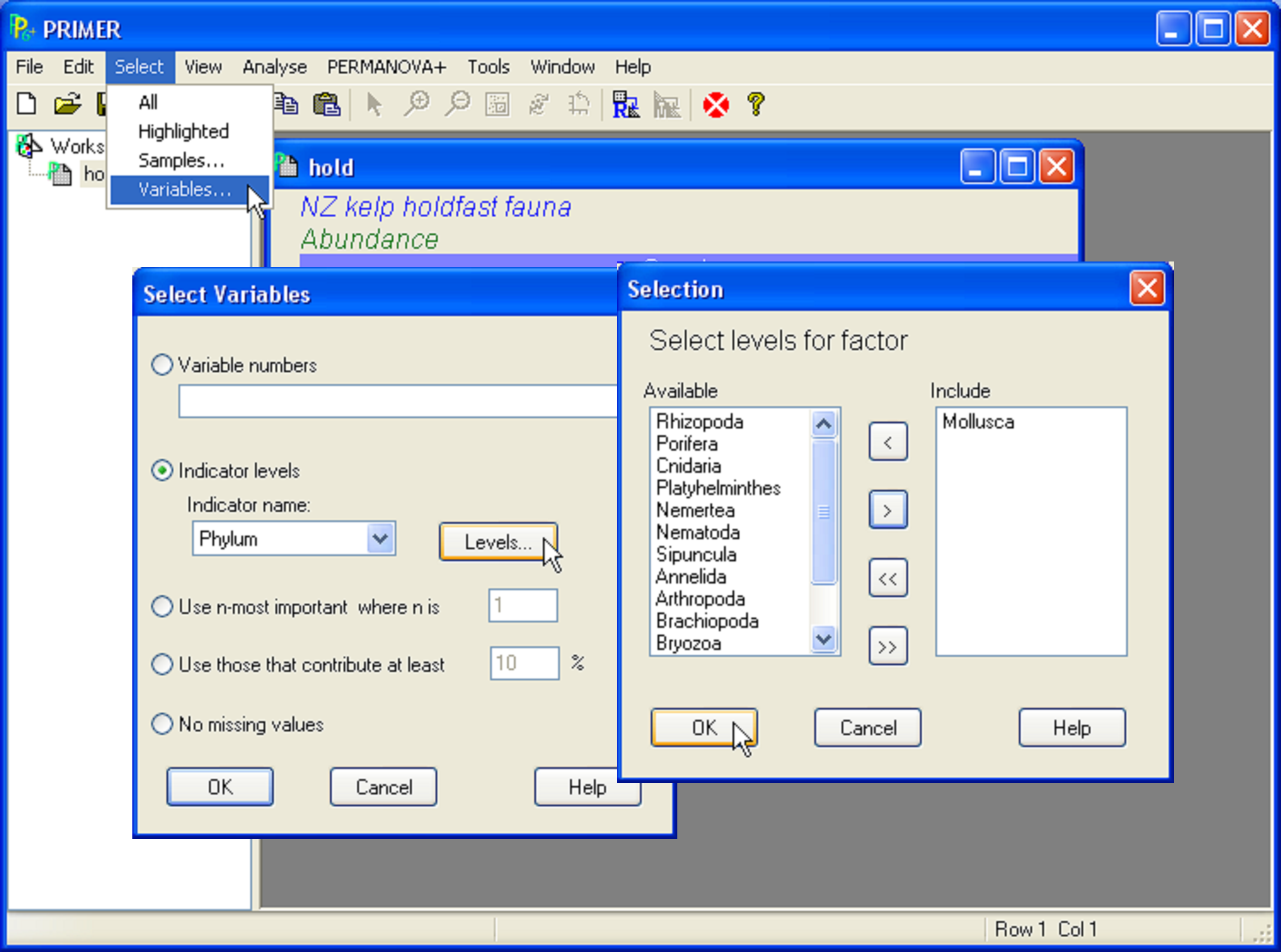Fig. 1.27. Dialog for selection of a subset of variables (molluscs only) for the holdfast data.

The objective here is to partition the variability in the species composition of molluscs according to the three-factor hierarchical experimental design. With our focus, for the moment, on composition alone (presence/absence), we will base the analysis on the Jaccard measure, which (when expressed as a dissimilarity) is directly interpretable as the percentage of unshared species between two sample units. We wish to determine if there is significant variability among areas, among sites and among locations in the composition of the molluscan assemblage. Furthermore, if significant variability is detected at any of these levels, it would then be logical (and interesting) to estimate and compare the sizes of each component of variation, which correspond to these different spatial scales.

Click on the mollusc worksheet, then select Analyse > Resemblance > (Analyse between •Samples) & (Measure •More (tab)), click on the tab at the top of the dialog window that is labeled ‘More’, then choose (•Similarity P/A > S7 Jaccard) and click ‘OK’. Next, we need to create an appropriate design file for the analysis (Fig. 1.28). Highlight the resulting Jaccard resemblance matrix and select PERMANOVA+ > Create PERMANOVA design > (Title: NZ kelp holdfast molluscs) & (Number of factors: 3). With the design file open, in the first column, place the name of each factor into its appropriate row by double-clicking inside the cell (Location in row 1, Site in row 2 and Area in row 3). Next, in column 3 of the design file, specify that each of these factors is ‘Random’. Now, you will need to specify explicitly the nesting relationships among the factors. To specify that sites are nested within locations, double click inside the cell in row 2 (for Sites) and column 2 (headed ‘Nested in’). This will bring up a new dialog that allows you to choose the factor within which ‘Sites’ are nested. Click on Location in the ‘Available’ box, followed by to move it over into the ‘Include’ box, then click ‘OK’. Specify also that Area is nested in Site, using the same approach (Fig. 1.28)³³. When you are finished specifying the design, rename the design file Nested design and save the workspace created so far as hold.pwk.

Fig. 1.28. Creating the PERMANOVA design for the New Zealand holdfast data, including nesting.

To run the analysis, highlight the resemblance matrix, choose PERMANOVA+ > PERMANOVA > (Design worksheet: Nested design) & (Num. permutations: 9999), leaving all other options as the defaults. The results show significant variability at each level in the design (Fig. 1.29). The EMS’s reveal the rationale for constructing correct pseudo-F ratios for each term in the model (Fig. 1.29).

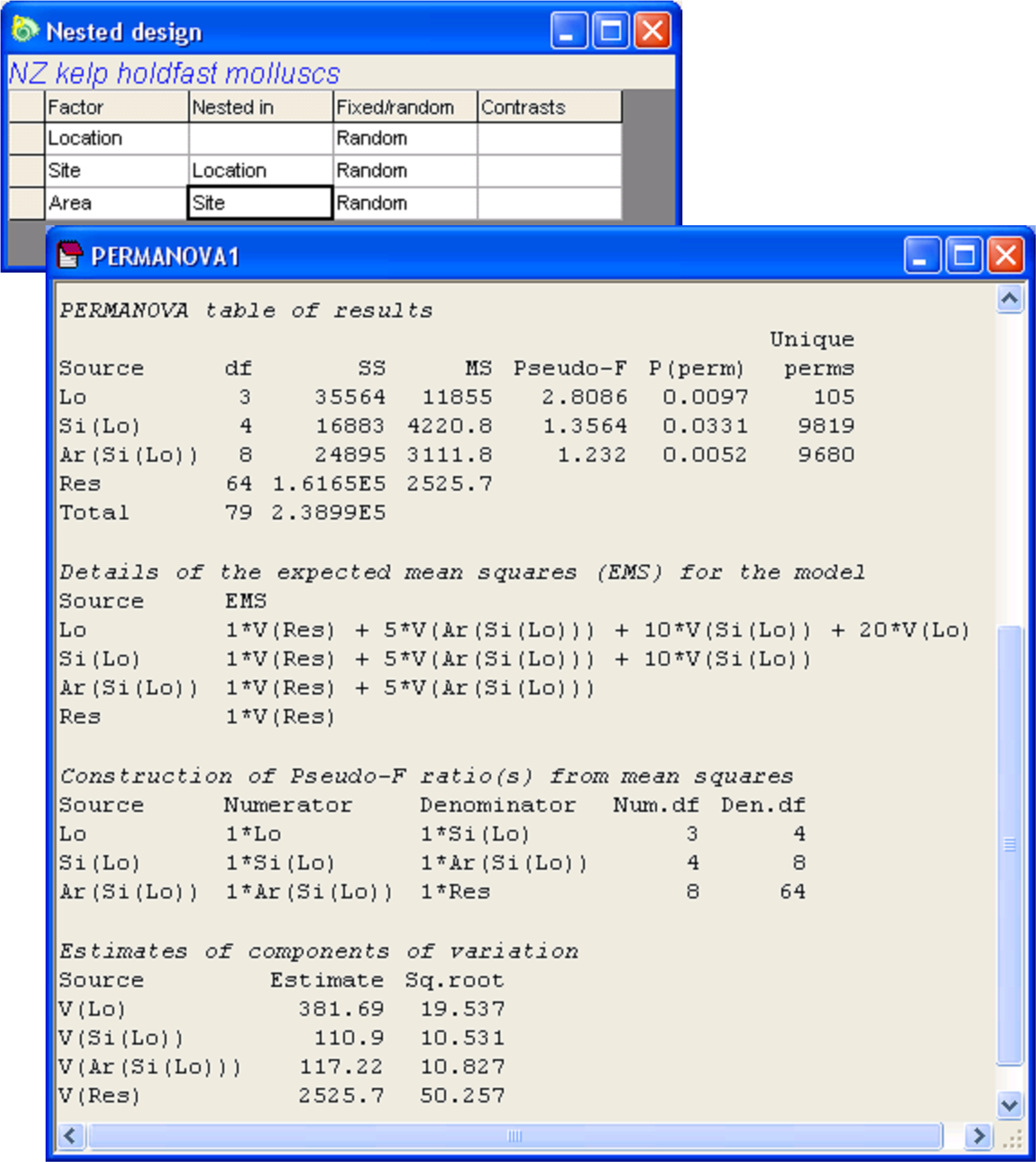Fig. 1.29. Design file and PERMANOVA analysis of variability in mollusc composition (based on the Jaccard measure) from kelp holdfast assemblages.

---

³² A holdfast is a root-like structure at the base of the kelp that holds it to the substratum, which is usually a rocky reef. A great diversity of invertebrates inhabit the interstices of these complex structures.

³³ PERMANOVA will do the correct analysis here if we choose to nest Areas within Sites only (because Sites have already been specified as being nested in Locations), as shown, or if we choose to specify explicitly that Areas are nested in Sites and also in Locations.