5.9 Caveats on using CAP (Tikus Island corals)

When using the CAP routine, it should come as no surprise that the hypothesis (usually) is evident in the plot. Indeed the role of the analysis is to search for the hypothesis in the data cloud. However, once faced with the constrained ordination, one might be tempted to ask the question whether it is useful to examine an unconstrained plot at all. The answer is most certainly ‘yes’! We would argue that it is always important to examine an unconstrained plot (either a PCO or an MDS if dealing with general resemblances, or a PCA if Euclidean distances are appropriate). There are several reasons for this.

First, a CAP plot (or other constrained plot, such as a dbRDA) views the data cloud through the filter of our hypothesis, so-to-speak, which is a bit like viewing the data through “rose-coloured glasses”, as mentioned before. This will have a tendency to lead us down the path towards an over-emphasis on the importance of the hypothesis, and we can easily neglect to put this into a broader perspective of the data cloud as a whole. Although a restriction on the choice of m and the use of cross-validation to avoid over-parameterising the problem will help to reduce this unfortunate instinct in us (i.e., our intrinsic desire to see our hypothesis in our data), the unconstrained plot has the important quality of “letting the data speak for themselves”. As the unconstrained plot does not include our hypothesis in any way to draw the points (but rather uses a much more general criterion, like preserving ranks of inter-point resemblances, or maximizing total variation across the cloud as a whole), we can trust that if we do happen to see our hypothesis playing a role in the unconstrained plot (e.g., to separate groups), then it is probably a pretty important feature of the data. So, first of all, the unconstrained plot helps to place our hypothesis within a broader perspective. Of course, if we see the separation of groups clearly in the unconstrained plot, then it should come as no surprise that the CAP routine will also have no trouble finding axes that are good at discriminating the groups. Diagnostics (like cross-validation) are crucial, however, for telling us something about the actual distinctiveness of the groups in multivariate space.
 

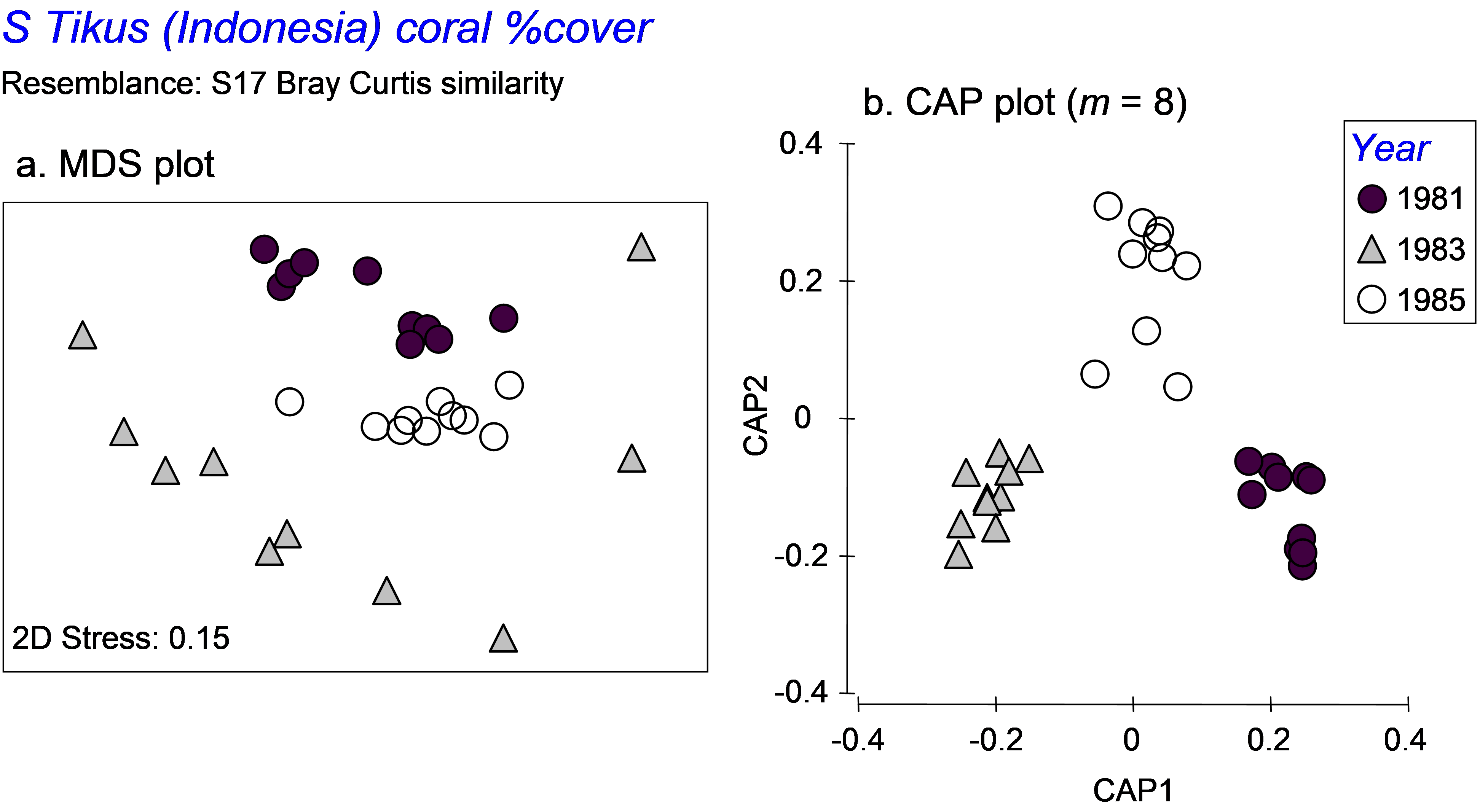Fig. 5.13. MDS and CAP plots for a subset of three years’ data on percentage cover of coral species from South Tikus Island, Indonesia.

Second, the purpose of the CAP routine is to seek out separation of the group centroids. As a consequence, it effectively completely ignores, and even destroys, differences in dispersions among the groups. A case in point serves as a useful example here. We shall re-visit the Tikus Island corals dataset (tick.pri in the ‘Corals’ folder of the ‘Examples v6’ directory), consisting of the percentage cover of p = 75 coral species in each of 6 years from 10 replicate transects in Indonesia ( Warwick, Clarke & Suharsono (1990) ). Taking only the years 1981, 1983 and 1985, we observed previously that the dispersions of these groups were very different when analysed using Bray-Curtis resemblances (Fig. 5.13a). However, when we analyse the data using CAP, the first two squared canonical correlations are very large (0.90 and 0.84, respectively), the cross-validation allocation success is impressively high (29/30 = 97%), and the plot shows the three groups of samples as very distinct from one another, with not even a hint of the differences in dispersions that we could see clearly before in the unconstrained MDS plot (Fig. 5.13b). These differences in dispersions are quite real (as verified by the PERMDISP routine), yet might well have remained completely unknown to us if we had neglected to examine the unconstrained plot altogether. An important caveat on the use of the CAP routine is therefore to recognise that CAP plots generally tell us absolutely nothing about relative dispersions among the groups. Only unconstrained plots (and associated PERMDISP tests) can do this.