4.3 Partitioning

Consider an (N × p) matrix of response variables Y, where N = the number of samples and p = the number of variables. Consider also an (N × q) matrix, X, which contains q explanatory (predictor) variables of interest (e.g. environmental variables). The purpose of DISTLM is to perform a permutational test for the multivariate null hypothesis of no relationship between matrices Y and X on the basis of a chosen resemblance measure, using permutations of the samples to obtain a P-value. In essence, the purpose here is to ask the question: does X explain a significant proportion of the multivariate variation in the data cloud described by the resemblance matrix obtained from Y (Fig. 4.1)? Note that the analysis done by DISTLM is directional and that these sets of variables have particular roles. The variables in X are being used to explain, model or predict variability in the data cloud described by the resemblance matrix arising from Y.
 

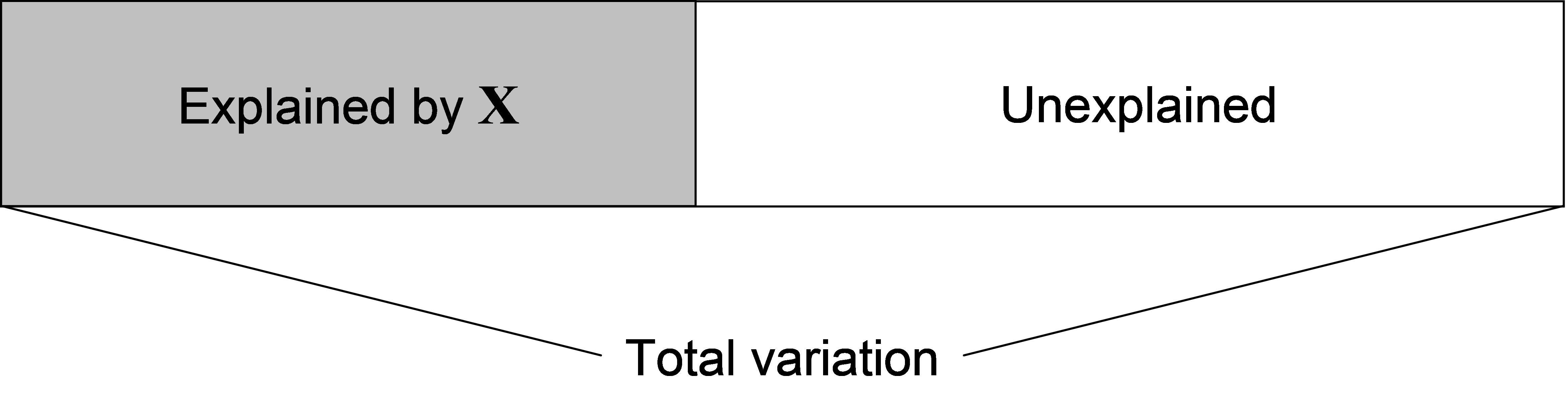
Fig. 4.1. Conceptual diagram of regression as a partitioning of the total variation into a portion that is explained by the predictor variables in matrix X, and a portion that is left unexplained (the residual).

Details of how dbRDA is done are provided by Legendre & Anderson (1999) and McArdle & Anderson (2001) . Maintaining a clear view of the conceptual framework is what matters most (Fig. 4.1), but a thumbnail sketch of the matrix algebra involved in the mechanics of dbRDA is also provided here. Suppose that D is an N × N matrix of dissimilarities (or distances) among samples⁷⁵. The analysis proceeds through the following steps (Fig. 4.2):

1. From the matrix of dissimilarities, D, calculate matrix A, then Gower’s centred matrix G, as outlined in steps 1 and 2 for doing a PCO (see Fig. 3.1);

2. The total sum of squares ($SS _{ \text{Total}}$) of the full multivariate data cloud is the sum of the diagonal elements (called the “trace” and symbolised here by “tr”) of matrix G, that is, tr(G);

3. From matrix X, calculate the “hat” matrix H = X[X′X]$^ {-1}$X′. This is the matrix derived from the solutions to the normal equations ordinarily used in multiple regression (e.g., Johnson & Wichern (1992) , Neter, Kutner, Nachtsheim et al. (1996) )⁷⁶;

4. The explained sum of squares for the regression ($SS _{ \text{Regression}}$) is then calculated directly as tr(HGH);

5. The unexplained (or residual) sum of squares is then $SS _{ \text{Residual}} = SS _{ \text{Total}} – SS _{ \text{Regression}}$. This is also able to be calculated directly as tr([I – H]G[I – H]), where I is an N × N identity matrix⁷⁷.

Fig. 4.2. Schematic diagram of distance-based redundancy analysis as performed by DISTLM.

Once the partitioning has been done, the proportion of the variation in the multivariate data cloud that is explained by the variables in X is calculated as: $$ R ^ 2 = \frac{ SS _{ \text{Regression}} }{ SS _{ \text{Total}}} \tag{4.1} $$ Furthermore, an appropriate statistic for testing the general null hypothesis of no relationship is: $$ F = \frac{ SS _{ \text{Regression}} / q}{ SS _{ \text{Residual}} / (N - q -1)} \tag{4.2} $$

This is the pseudo-F statistic, as already seen for the ANOVA case in chapter 1 (equation 1.3). It is a direct multivariate analogue of Fisher’s F ratio used in traditional regression. However, when using DISTLM, we do not presume to know the distribution of pseudo-F in equation 4.2, especially for p > 1 and where a non-Euclidean dissimilarity measure has been used as the basis of the analysis. Typical values we might expect for pseudo-F in equation (4.2) if the null hypothesis of no relationship were true can be obtained by randomly re-ordering the sample units in matrix Y (or equivalently, by simultaneously re-ordering the rows and columns of matrix G), while leaving the ordering of samples in matrix X (and H) fixed. For each permutation, a new value of pseudo-F is calculated (F$ ^ \pi$). There is generally going to be a very large number of possible permutations for a regression problem such as this; a total of N! (i.e., N factorial) re-orderings are possible. A large random subset of these will do in order to obtain an exact P-value for the test ( Dwass (1957) ) . The value of pseudo-F obtained with the original ordering of samples is compared with the permutation distribution of F$ ^ \pi$ to calculate a P-value for the test (see equation 1.4 in chapter 1).

If Euclidean distances are used as the basis of the analysis, then DISTLM will fit a traditional linear model of Y versus X, and the resulting F ratio and R$^2$ values will be equivalent to those obtained from:

• a simple regression (when p = 1 and q = 1);

• a multiple regression (when p = 1 and q > 1); or

• a multivariate multiple regression (when p > 1 and q > 1). Traditional multivariate multiple regression is also called redundancy analysis or RDA (Gittins 1985, ter Braak 1987).

An important remaining difference, however, between the results obtained by DISTLM compared to other software for such cases is that all P-values in DISTLM are obtained by permutation, thus avoiding the usual traditional assumption that errors be normally distributed.

The added flexibility of DISTLM, just as for PERMANOVA, is that any resemblance measure can be used as the basis of the analysis. Note that the “hat” matrix (H) is so-called because, in traditional regression analysis, it provides a projection of the response variables Y onto X ( Johnson & Wichern (1992) ) transforming them to their fitted values, which are commonly denoted by $\hat{\text{\bf Y}}$ . In other words, we obtain fitted values (“y-hat”) by pre-multiplying Y by the hat matrix: $\hat{\text{\bf Y}} = \text{\bf HY}$. Whereas in traditional multivariate multiple regression the explained sum of squares (provided each of the variables in Y are centred on their means) can be written as tr($\hat{\text{\bf Y}}$ $\hat{\text{\bf Y}}^ \prime$ )=tr(HYY$^\prime$H), we achieve the ability to partition variability more generally on the basis of any resemblance matrix simply by replacing YY$^\prime$ in this equation with G ( McArdle & Anderson (2001) ). If Euclidean distances are used in the first place to generate D, then G and YY$^ \prime$ are equivalent⁷⁸ and DISTLM produces the same partitioning as traditional RDA. However, if D does not contain Euclidean distances, then G and YY$^ \prime$ are not equivalent and tr(HGH) produces the explained sum of squares for dbRDA on the basis of the chosen resemblance measure.

Two further points are worth making here about dbRDA and its implementation in DISTLM.

• First, as should be clear from the construction of the pseudo-F statistic in equation 4.2, the number of variables in X(q) cannot exceed (N – 1), or we simply run out of residual degrees of freedom! Furthermore, if q = N – 1, then we will find that $R ^ 2$ reaches its maximum at 1.0, meaning the percentage of variation explained is 100%, even if the variables in X are just random numbers! This is a consequence of the fact that $R ^ 2$ always increases with increases in the number of predictor variables. It is always possible to find a linear combination of (N – 1) variables (or axes) that will fit N points perfectly (see the section Mechanics of PCO in chapter 3). Thus, if q is large relative to N, then a more parsimonious model should be sought using appropriate model selection criteria (see the section Building models below).

• Second, the method implemented by DISTLM, like PERMANOVA but in a regression context, provides a true partitioning of the variation in the data cloud, and does not suffer from the problems identified for partial Mantel tests identified by Legendre, Borcard & Peres-Neto (2005) . The partial Mantel-type methods “expand” the resemblance matrix by “unwinding” it to a total of N(N – 1)/2 different dissimilarity units. These are then (unfortunately) treated as independent samples in regression models. In contrast, the units being treated as independent in dbRDA are the original individual samples (the N rows of Y, say), which are the exchangeable units under permutation. Thus, the inherent structure (the correlation among variables and the values within a single sample row) and degree of non-independence among values in the resemblance matrix remain intact under the partitioning and permutation schemes of dbRDA (whether it is being implemented using the PERMANOVA routine or the DISTLM routine), but this is not true for partial Mantel tests⁷⁹. See the section entitled SS from a distance matrix in chapter 1 for further discussion.

---

⁷⁵ If a resemblance matrix of similarities is available instead, then DISTLM in PERMANOVA+ will automatically transform these into dissimilarities; the user need not do this as a separate step.

⁷⁶ Regression models usually include an intercept term. This is obtained by including a single column of 1’s as the first column in matrix X. DISTLM automatically includes an intercept in all of its models. This amounts to centring the data before analysis and has no effect on the calculations of explained variation.

⁷⁷ An identity matrix (I) behaves algebraically like a “1” in matrix algebra. It is a square diagonal matrix with 1’s all along its diagonal and zeros elsewhere.

⁷⁸ This equivalence is noted on p. 426 of Legendre & Legendre (1998) and is also easy to verify by numerical examples.

⁷⁹ An interesting point worth noting here is to consider how many df are actually available for a multivariate analysis. If p = 1, then we have a total of N independent units. If p > 1, then if all variables were independent of one another, we would have N × p independent units. We do not expect, however, to have independent variables, so, depending on their degree of inter-correlation, we expect the true df for the multivariate system to lie somewhere between N and N × p. The Mantel-type procedure, which treats with N(N – 1)/2 units is generally going to overestimate the true df, or information content of the multivariate system, while PERMANOVA and dbRDA’s use of N is, if anything, an underestimate. This is clearly an area that warrants further research.