4.15 Categorical predictor variables (Oribatid mites)

Sometimes the predictor variables of interest are not quantitative, continuous variables, but rather consist of categories or groups, called categorical or nominal variables. There are also situations where we have mixtures of variable types that we want to include in a single DISTLM analysis. For example, we might want to consider a single model that includes temperature and salinity (continuous and quantitative) but which also includes a categorical variable, habitat, that might be recorded for each sample as one out of a number of different types: sand, coral, rock, seagrass, etc. How can we analyse categorical predictor variables using DISTLM?

As an example, we will consider an analysis of environmental control and spatial structure in an oribatid mite community, described by Borcard, Legendre & Drapeau (1992) and Borcard & Legendre (1994) . These data come from a site adjacent to a small Laurentide lake, Lake Geai, at the Station de Biologie des Laurentides in Quebec, Canada. The species (response) data (in the file ormites.pri in the ‘OrbMit’ folder of the ‘Examples add-on’ directory) consist of counts of abundances for each of p = 35 species of oribatid mites from each of N = 70 sites. The file orenvgeo.pri (in the same folder) contains a number of predictor variables associated with each of the sites. Some of these are spatial variables and correspond to the geographic coordinates of each sample on a grid measured in metres (‘x’, ‘y’) and up to third-order polynomial functions of these (‘x2’, ‘xy’, ‘y2’, etc.). The others are environmental variables, which include two quantitative variables:

• Substratum density (‘Substr.dens’), measured in grams per litre of dry uncompressed matter, and

• Water content of the substratum (‘H20.cont’), measured in grams per litre, and three categorical (nominal) variables:

• Substrate (7 categories: Sphagnum groups 1-4, litter, bare peat, interfaces),

• Shrubs (3 categories: no shrubs, few shrubs, many shrubs), and

• Microtopography (2 categories: blanket (flat) and hummock (raised))

The nominal variable ‘Shrubs’ is actually ordinal or semi-quantitative, so the simple rank order values of ‘1’, ‘2’ and ‘3’ in a single column could also be used here to treat this as a single (1 df) continuous quantitative predictor variable. However, we shall treat it as a nominal variable here to be consistent with the way this variable was treated by Borcard, Legendre & Drapeau (1992) and Borcard & Legendre (1994) .

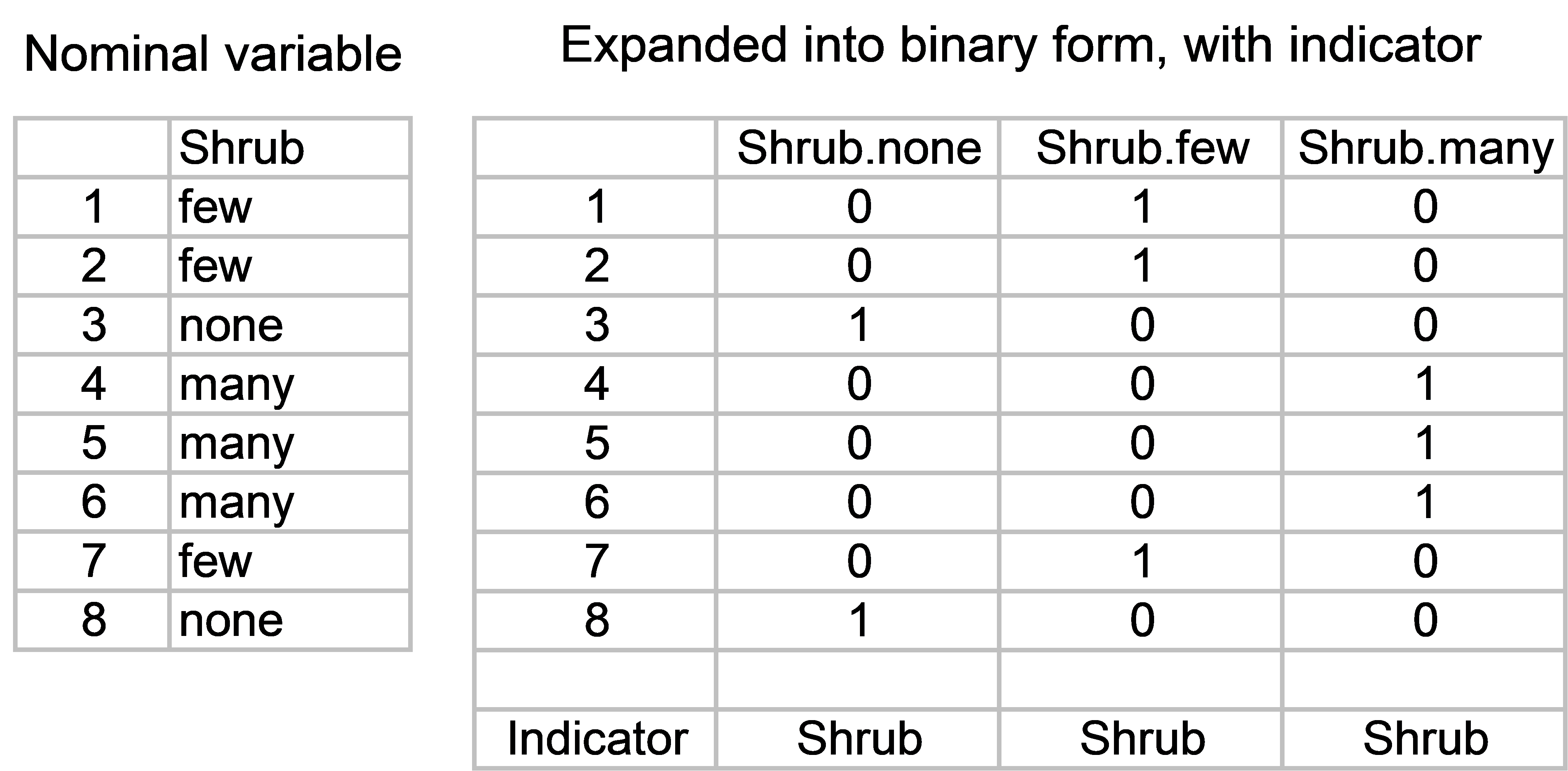
Fig. 4.22. Example of a categorical (nominal) variable and its expanded binary form.

To start with, we need to expand each categorical variable of interest into a set of “on/off” or binary variables (e.g., Fig. 4.22). For each categorical variable, there will be as many binary variables as there are categories. The binary variables will take a value of ‘1’ for samples where that category occurs, and zero (‘0’) elsewhere. Once this has been done, the binary variables associated with a particular nominal variable need to be specified as a set, using an indicator in PRIMER (see the previous section on setting up indicators to analyse sets of variables). For example, the seven “on/off” variables that “code” for each of the seven substrate categories are identified (by having a common name for the indicator) as belonging to the ‘Substrate’ set. If there are also quantitative variables to be analysed as part of the same predictor variable worksheet, then each of these can simply be specified in the indicator as belonging to its own “set”. The environmental data, with the categorical variables already expressed as binaries and identified in sets using the indicator called ‘Type’, are located in the file orenvgeo.pri (Fig. 4.23).

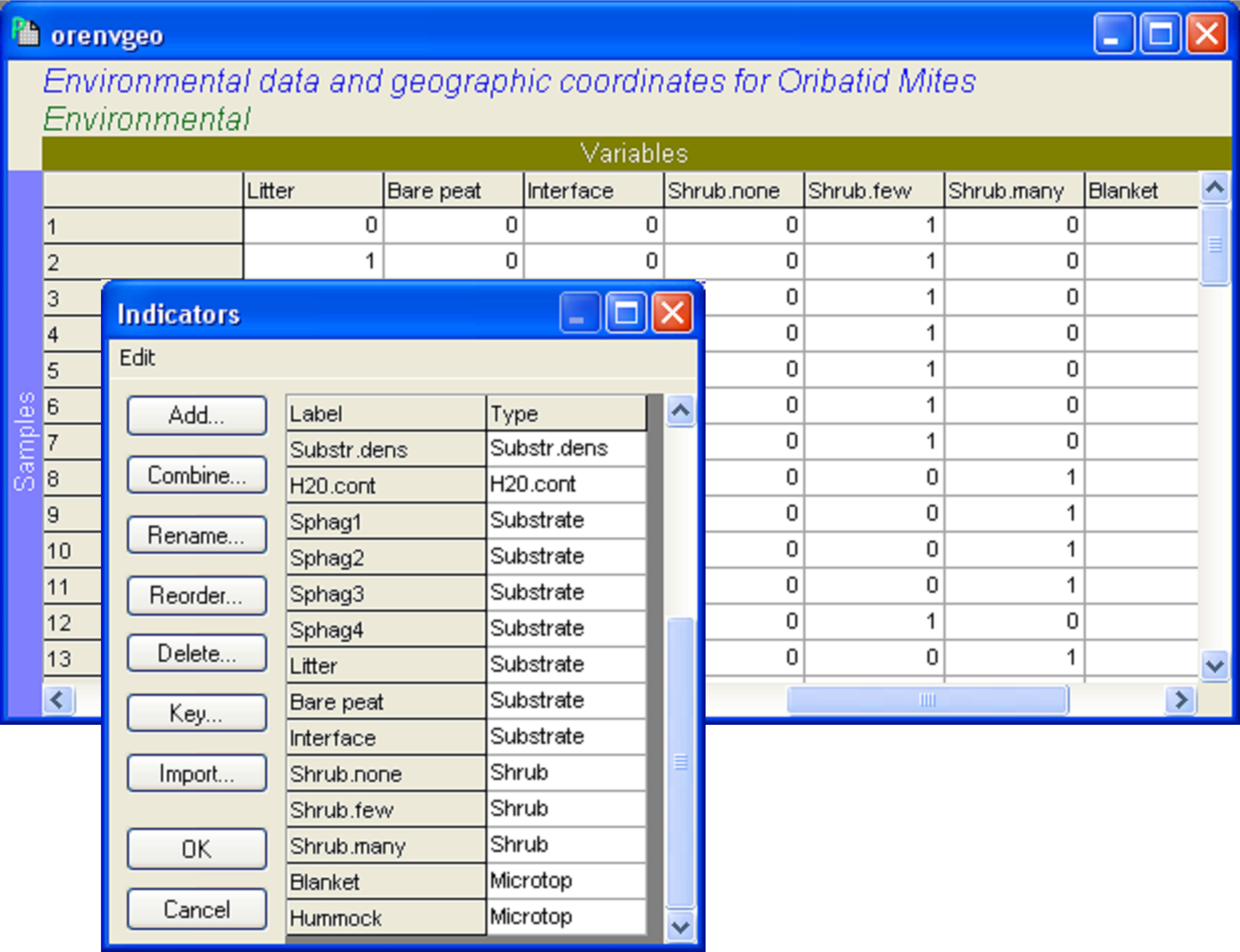
Fig. 4.23. Environmental variables in binary form and their indicator (‘Type’) for the oribatid mite data set.

The df for each categorical set is the number of categories minus 1. Each quantitative variable has one degree of freedom (= 1 df) associated with it for a regression. Another way of thinking about this is that we have to estimate one slope parameter (or coefficient) for each quantitative variable we wish to include in the model. When we have a categorical variable, however, the number of degrees of freedom associated with it is the number of categories minus 1. The reason for the “minus 1” becomes clear when we think about the way the binary “codes” for a given set are specified. Consider a categorical variable that has two categories, like ‘Microtopography’ in the oribatid mite example. Once you are given the first binary variable ‘Blanket’, you automatically know what the other binary variable must be: ‘Hummock’ will have 1’s wherever ‘Blanket’ has zeros, and vice versa. Therefore, the variable ‘Hummock’ is actually completely redundant here. This issue⁹⁴ is also readily seen by calculating the correlation between ‘Blanket’ and ‘Hummock’, r = -1.0, a perfect negative correlation! So one (or the other) of these variables needs to be removed for the analysis. Fortunately, the DISTLM routine automatically determines the correct degrees of freedom for a given set of variables and will omit unnecessary variables, even when all of the binary variables have been included by the user.

As an aside, analysis of variance is simply a regression on categorical variables. Therefore, we can actually do PERMANOVA-style analyses using DISTLM by setting up ‘binary codes’ for each of the factors (as in Fig. 4.22). With the PERMANOVA+ tool at our disposal, however, it is much more efficient to analyse the responses of multivariate variables to an ANOVA design using the PERMANOVA routine instead, as this already caters for balanced and unbalanced designs with or without quantitative (or categorical) covariables. PERMANOVA also allows factors to be nested within other factors and correctly analyses random factors and mixed models, whereas DISTLM will treat all of the predictor variables (whether they be quantitative or categorical) as fixed⁹⁵. In some sense, it may seem odd to treat quantitative predictor variables as if they are “fixed”. In many ecological applications, for example, a scientist has measured the X predictor variables (say, a suite of environmental variables) for each sample in much the same way as the Y response variables (say, abundances or counts of species). So arguably the X variables should be modeled with error, just as the Y variables are (e.g., McArdle (1988) , Warton & Weber (2002) , McArdle (2003) , Warton, Wright, Falster et al. (2006) ). Another way of viewing the regression approach, however, is not so much that the X variables are measured without error, but rather that the models we construct from them are conditional on the actual values we happened to observe (e.g., Neter, Kutner, Nachtsheim et al. (1996) ). One natural consequence of this philosophical stance (among others) is that it is not appropriate to extrapolate the resulting models beyond the range of observed values of X, a well-known caveat for regression.

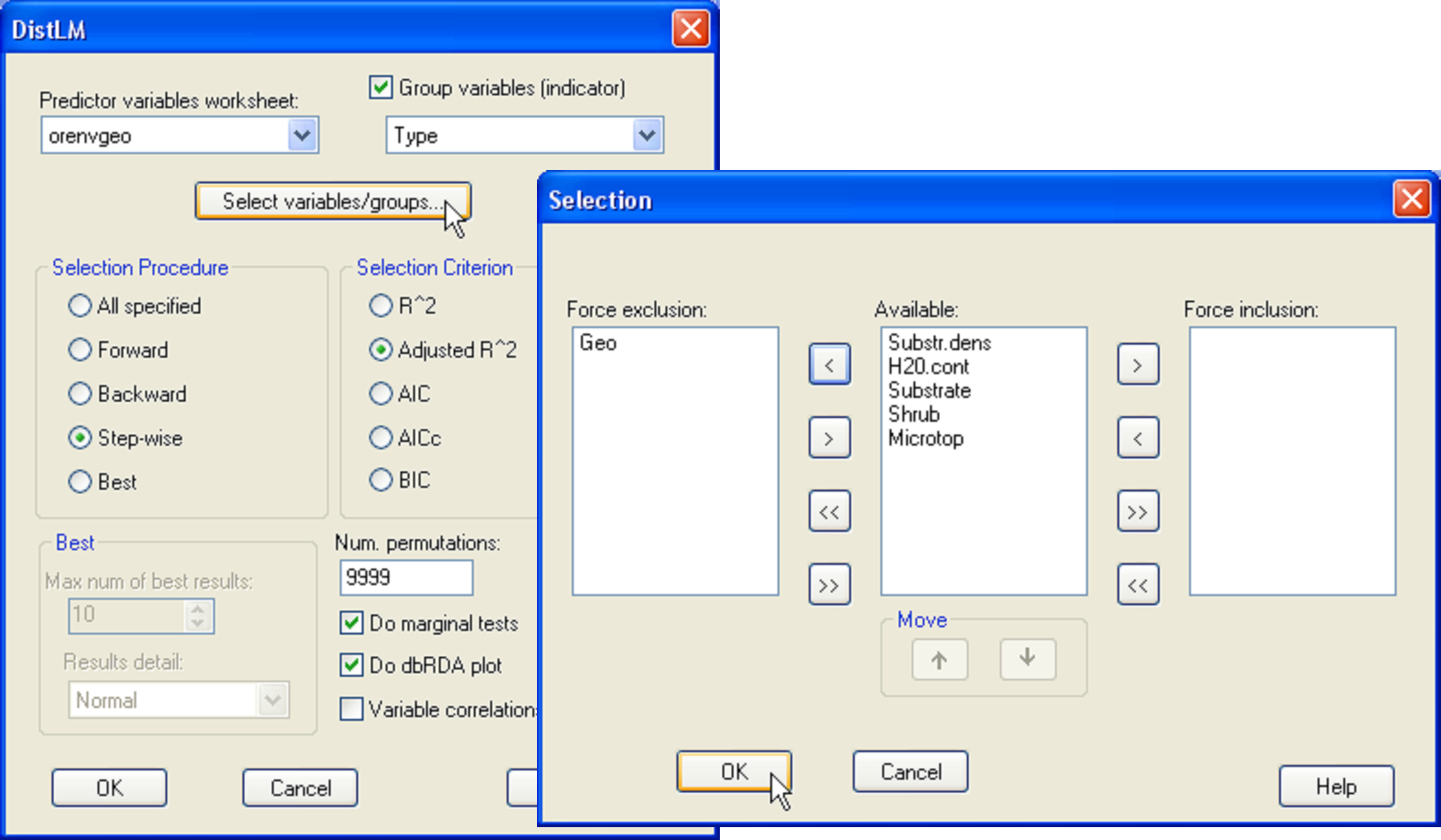
Fig. 4.24. DISTLM dialog for fitting the environmental variables (a mixture of quantitative and categorical variables) to the oribatid mite data, while excluding the geospatial variables.

Returning to the example, for simplicity we shall restrict our attention to the environmental variables only and omit the spatial variables from the analysis in what follows. The distributions of the categorical variables need not be considered using the usual diagnostic tools, as these only consist of 1’s and 0’s. A scatter plot using the draftsman plot tool in PRIMER for the two quantitative predictor variables alone (‘H2O.cont’ and ‘Substr.dens’) shows fairly even scatter and no indication that either of these variables requires any transformation prior to analysis. So, we are ready to proceed. First, calculate a Bray-Curtis resemblance matrix after square-root transforming the oribatid mite species abundance data. From this resemblance matrix, choose PERMANOVA+ > DISTLM > (Predictor variables worksheet: orenvgeo) & ($\checkmark$Group variables (indicator) Type) & (Selection Procedure •Step-wise) & (Selection Criterion •Adjusted R^2) & (Num. permutations: 9999) & ($\checkmark$Do marginal tests) & ($\checkmark$Do dbRDA plot). Before clicking the ‘OK’ button for the DISTLM dialog, force the exclusion of the spatial variables by clicking on the ‘Select variables/groups’ button and moving the group ‘Geo’ over into the ‘Force exclusion:’ column of the ‘Selection’ dialog (Fig. 4.24). The choice of adjusted R$^2$ as the selection criterion for this case is especially appropriate, because this criterion will take into account the fact that the sets of predictor variables have different numbers of variables in them, whereas the use of the raw R$^2$ criterion will not. If model selection were the ultimate aim, then one might alternatively choose to use AIC or BIC instead, which also would take into account the different numbers of variables in different sets. In our case, interest lies in determining how much of the variability is explained by each set of variables (thus the choice to examine marginal tests), and also what a sequential step-wise model fit of these sets of variables would produce.

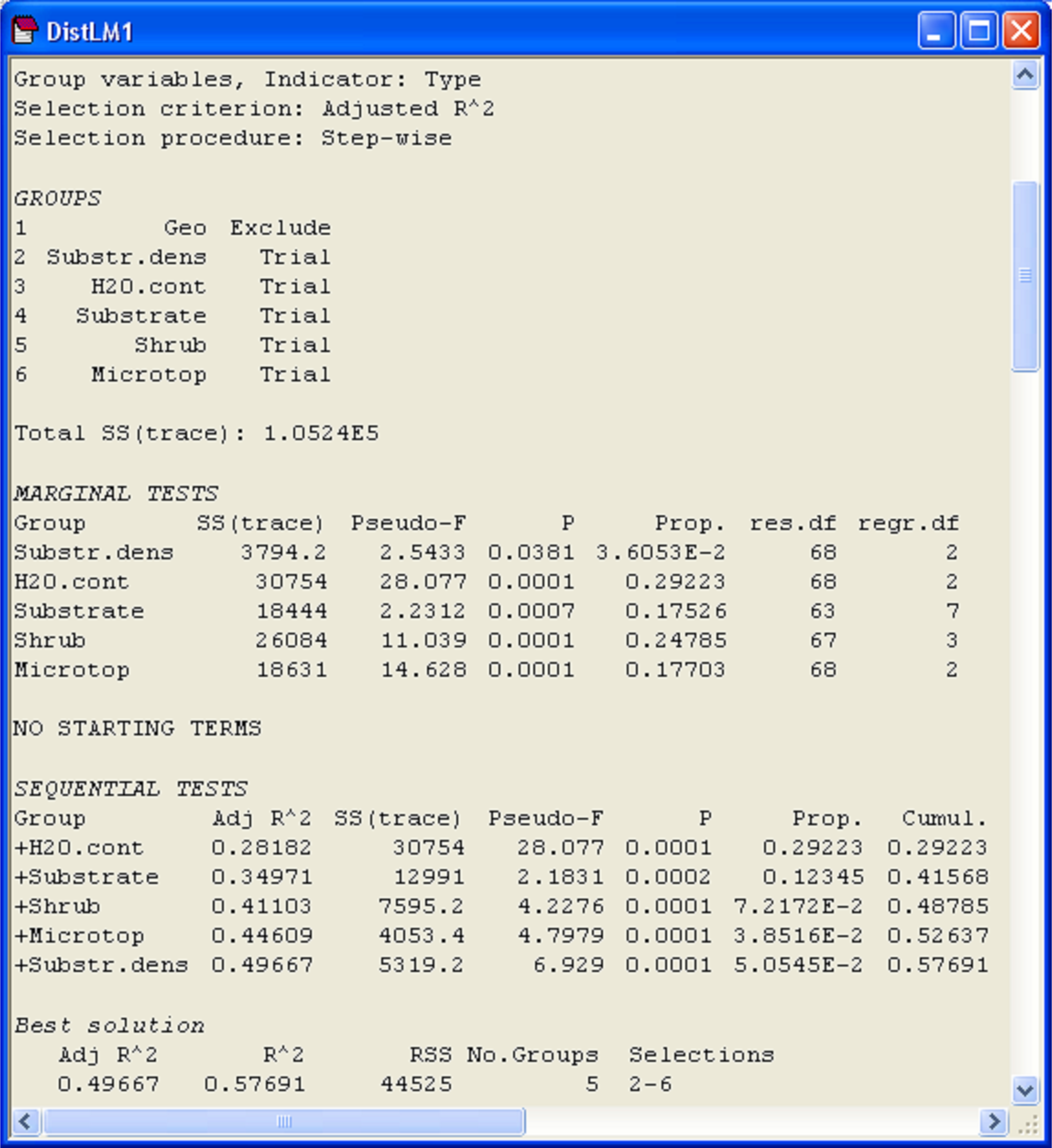
Fig. 4.25. Results of DISTLM for fitting the environmental variables (a mixture of quantitative and categorical variables) to the oribatid mite data, while excluding the geospatial variables.

Marginal tests (Fig. 4.25) show that each of the sets explains a significant proportion of the variation in the mite data, when considered alone (P < 0.05 in all cases). The single variable of water content (‘H2O.cont’) alone explains the greatest amount of variation in the oribatid mite species data cloud (based on Bray-Curtis), at 29.2%, while substrate density explains the least (only 3.6%). The set of variables that increased the value of adjusted R$^2$ the most after fitting ‘H2O.cont’ was ‘Substrate’, followed by ‘Shrub’, ‘Microtop’ and then ‘Substr.dens’. Although a step-wise procedure was used, at no stage were there any eliminations of sets from the model once they had been added and the conditional tests associated with each of the sequential additions were statistically significant (P < 0.001 in all cases). All of these predictor variables together explained 57.7% of the variation in the species data cloud and the adjusted R$^2$ for the full model was 0.497 (Fig. 4.25).

The full model can be visualised by examining the dbRDA ordination, requested as part of the output. The first two dbRDA axes captured nearly 80% of the variability in the fitted model, 45.7% of the total variation in the data cloud (Fig. 4.26). The vector overlay shows how the first dbRDA axis is particularly strongly related to water content, shrubs (none versus many) and microtopography (blanket versus hummock). When categorical variables are included in a DISTLM analysis, then the length of each categorical vector is a measure of the strength of the relationship between that category and the dbRDA axes. More particularly, if the separation of groups is clear in the plot, then we would expect the vectors for those categories to be relatively long. To help interpret ordination plots, it may be useful to provide the categorical variables also as factors; this will allow labels and symbols to be placed on the plot according to these different groupings. For example, by superimposing symbols corresponding to the three categories of ‘Shrubs’, a gradient from ‘none’ to ‘many’ (left to right) is apparent in the dbRDA diagram (Fig. 4.26). We leave it to the user to explore other categorical variables in this way, to examine unconstrained ordinations for the oribatid mite data and to consider analyses that might include the spatial variables as well.

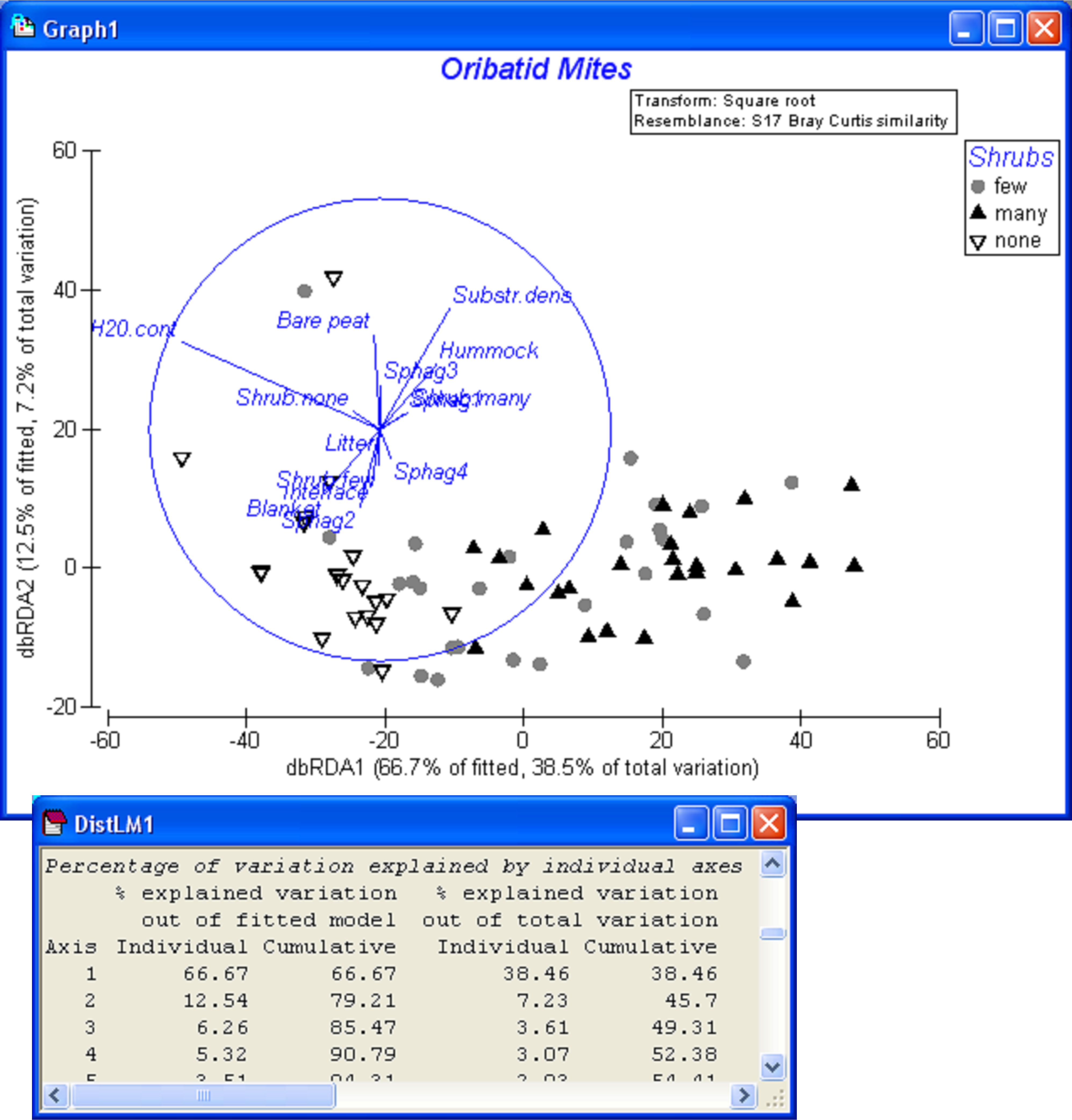
Fig. 4.26. dbRDA ordination for the fitted model of oribatid mite data (based on Bray-Curtis after square-root transformation of abundances) versus environmental variables.

---

⁹⁴ This phenomenon is sometimes referred to as the “overparameterisation” of an ANOVA model.

⁹⁵ The treatment of quantitative predictor variables as random (sometimes called “Model II” regression) does not exist within the current framework of either PERMANOVA or DISTLM and is a topic for further research. The CAP routine, however, is designed to examine the canonical correlations between two (sphericised) data clouds; it can be considered as one type of multivariate analogue to Model II regression. See chapter 5 for details.