5.5 Diagnostics
How did the CAP routine choose an appropriate number of PCO axes to use for the above discriminant analysis (m = 7)? The essential idea here is that we wish to include as much of the original variability in the data cloud as possible, but we do not wish to include PCO axes which do nothing to enhance our ability to discriminate the groups. To do so would be to look at the problem with “rose-coloured” glasses. Indeed, if we were to use all of the PCO axes, then the canonical plot will just show our hypothesis back at us again, which is useless. Recall that in CAP, we are using the PCO axes to predict the groups, and a linear combination of (N – 1) PCO axes can easily be used to plot N points according to any hypothesis provided in X perfectly. For example, if we choose m = 55 for the above example (as N = 56), we will see a CAP plot with the samples within each of the three different groups superimposed on top of one another onto three equidistant points. This tells us nothing, however, about how distinct the groups are in the multivariate space, nor how well the PCO axes model and discriminate among the groups, particularly given a new observation, for example. One appropriate criterion for choosing m is to choose the number of axes where the probability of misclassifying a new point to the wrong group is minimised.
To estimate the misclassification error using the existing data, we can use a leave-one-out procedure ( Lachenbruch & Mickey (1968) , Seber (1984) ). The steps in this procedure are:
-
Take out one of the points.
-
Do the CAP analysis without it.
-
Place the “left-out” point into the canonical space produced by the others.
-
Allocate the point to the group whose centroid (middle location) is closest to it.
-
Was the allocation successful? (i.e., did the CAP model classify the left-out point to its correct group?)
-
Repeat steps 1-5 for each of the points.
-
Misclassification error = the proportion of points that were misclassified. The proportion of correct allocations is called allocation success (= 1 minus the misclassification error).
By repeating this for each of a series of values for m, we can choose to use the number of axes that minimises the misclassification error. Although not a strict requirement, we should also probably choose m to be at least as large so as to include ~ 60% of the variation in the original resemblance matrix (if not more). The CAP routine will go through the above outlined leave-one-out procedure for each value of m and will show these diagnostics in the output file103. For discriminant-type analyses, a value of m is chosen which maximises the allocation success (i.e., minimises the misclassification error). For canonical correlation-type analyses, the value of m is chosen which minimises the leave-one-out residual sum of squares. The user can also choose the value of m manually in the CAP dialog, with the option to do the diagnostics for this chosen value of m alone or for all values of m up to and including the value chosen (Fig. 5.4).
An output table of diagnostics is shown for the Poor Knights fish dataset in Fig. 5.7. For each value of m, the diagnostic values given are:
-
‘prop.G’ = the proportion of variation in the data cloud described by the resemblance matrix (represented in matrix G) explained by the first m PCO axes;
-
‘ssres’ = the leave-one-out residual sum of squares;
-
‘d_1^2’ = the size of the first squared canonical correlation ($\delta _1 ^2$);
-
‘d_2^2’ = the size of the second104 squared canonical correlation ($\delta _2 ^2$);
-
‘%correct’ = the percentage of the left-out samples that were correctly allocated to their own group using the first m PCO axes for the model.
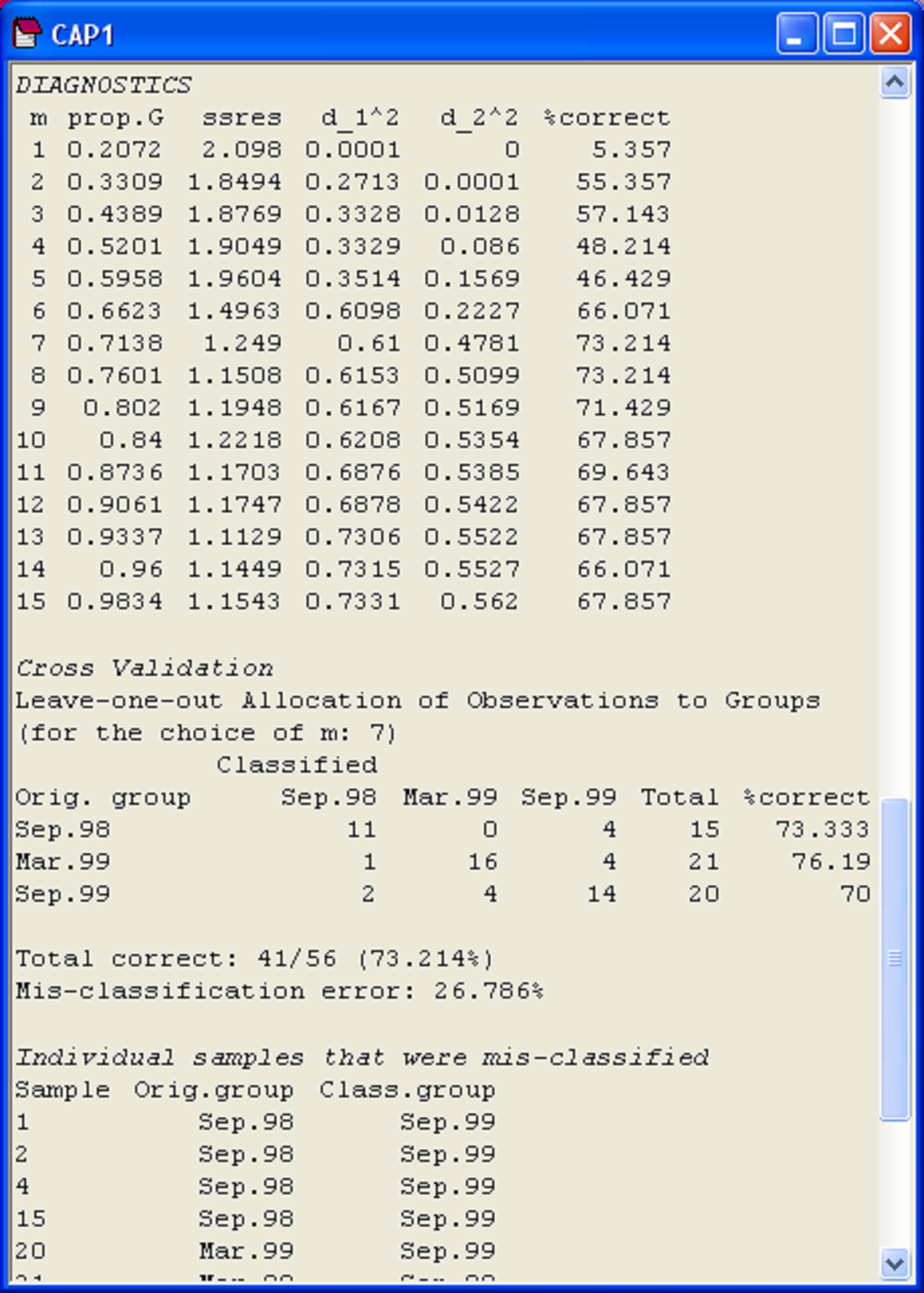 Fig. 5.7. Diagnostics and cross-validation results for the CAP analysis of the Poor Knights fish data.
It often helps to visualise these different diagnostics as a function of m, as shown in Fig. 5.8. First, we can see that the proportion of variation in the original data cloud that is explained by the first m PCO axes (Fig. 5.8a) is a smooth function of m, which is no surprise (as we saw before, the first 2 PCO axes explain 33.1% of the variation, see Fig. 5.3). Next, we can see that the values of the squared canonical correlations ($\delta _1 ^2$ and $\delta _2 ^2$), also just continue to increase, the more axes we choose to use. However, they do appear to pretty much “level-off” after m = 6 or 7 axes (Fig. 5.8b). So, we don’t get large increases or improvements in either of the canonical correlations by including more than m = 7 axes. Unlike the canonical correlations, neither the leave-one-out allocation success, nor the leave-one-out residual sum of squares has a monotonic relationship with m. Although the leave-one-out residual sum of squares is minimised when m = 13 (Fig. 5.7), we can see that no great reduction in its value is achieved beyond about m = 7 or 8 (Fig. 5.8c). Finally, the leave-one-out allocation success was maximised at m = 7, where 41 out of the 56 samples (73.2%) were allocated to the correct group using the CAP model (Fig. 5.8d). The CAP routine has chosen m = 7 based on this diagnostic alone, but the other diagnostic information also indicates that a value of m around 7 indeed would be appropriate for these data. These first 7 PCO axes explain about 71.4% of the total variation in tr(G) (‘prop.G’, Fig. 5.7). Although we would generally like this figure to be above 60% for the chosen value of m, as it is here, this is not a strict requirement of the analysis, and examples do exist where only the first one or two PCO axes are needed to discriminate groups, even though these may not necessarily include a large proportion of the original total variation.
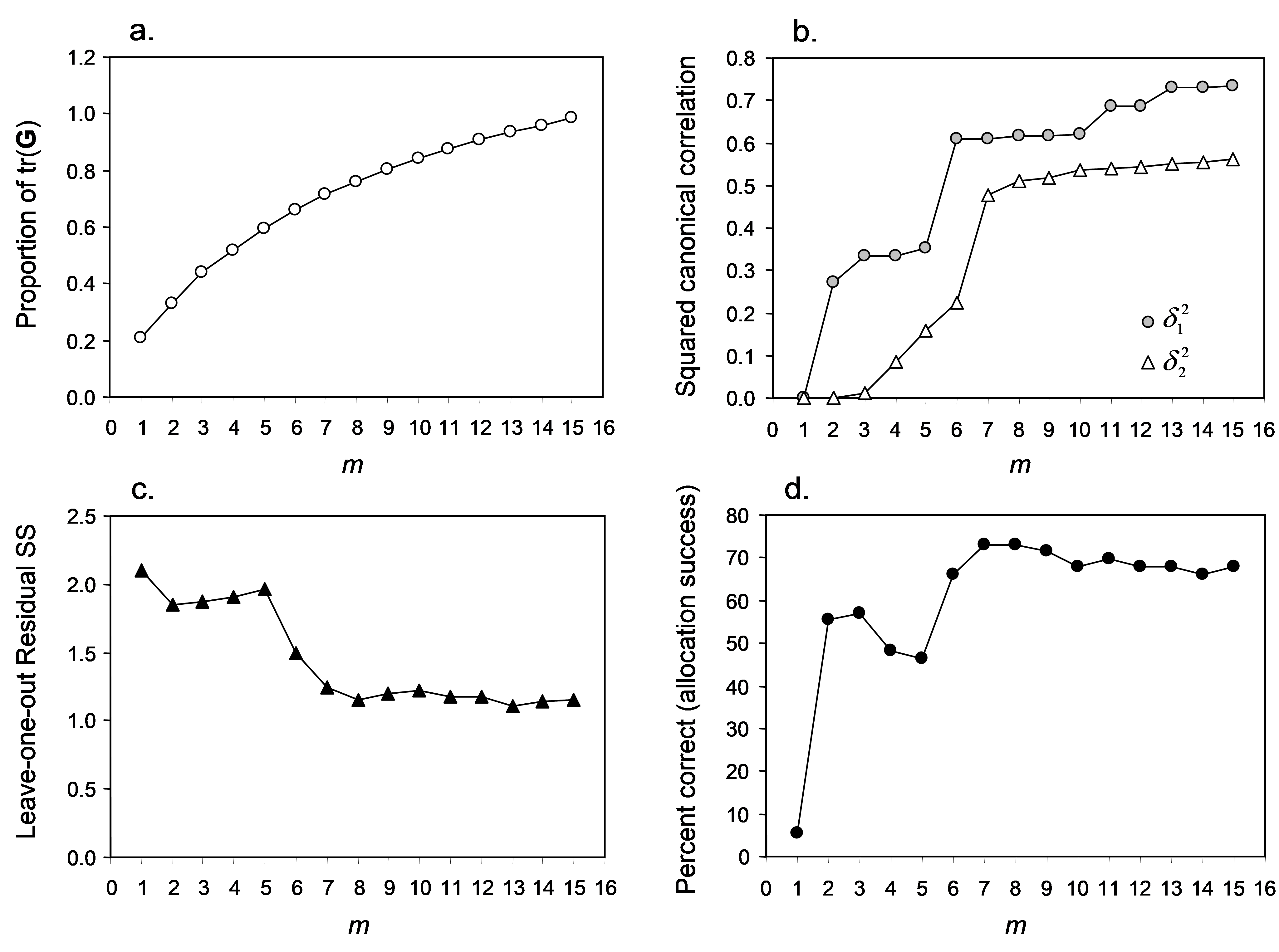 Fig. 5.8. Plots of individual diagnostic criteria for the CAP analysis of Poor Knights fish data.
Generally, the CAP routine will do a pretty decent job of choosing an appropriate value for m automatically, but it is always worthwhile looking at the diagnostics carefully and separately in order to satisfy yourself on this issue before proceeding. In some situations (namely, for data sets with very large N), the time required to do the diagnostics can be prohibitively long. One possibility, in such cases, is to do a PCO analysis of the data first to get an idea of what range of m might be appropriate (encapsulating, say, up to 60-80% of the variability in the resemblance matrix), and then to do a targeted series of diagnostics for individual manual choices of m to get an idea of their behaviour, eventually narrowing in on an appropriate choice.
103 The diagnostics will stop when CAP encounters m PCO axes that together explain more than 100% of the variation in the resemblance matrix, as will occur for systems that have negative eigenvalues (e.g., see Fig. 3.5). In the present case, the diagnostics do not extend beyond m = 15. Examination of the PCO output file for these data shows that the first 16 PCO axes explain 100.58% of the variation in tr(G).
104 There will be as many columns here as required to show all of the canonical eigenvalues – in the present example, there are only two canonical eigenvalues, so there are two columns for these.