1.14 Two-way crossed design (Subtidal epibiota)
The primary advantage of PERMANOVA is its ability to analyse complex experimental designs. The partitioning inherent in the routine allows interaction terms in crossed designs to be estimated and tested explicitly. As an example, consider a manipulative experiment done to test the effects of shading and proximity to the seafloor on the development of subtidal epibiotic assemblages in Sydney Harbour, Australia ( Glasby (1999) ). The data are located in the file sub.pri in the ‘SubEpi’ folder of the ‘Examples add-on’ directory. It was observed that assemblages colonising pilings at marinas were different from those colonising nearby natural sandstone rocky reefs. Glasby (1999) proposed that this difference might be due to the fact that assemblages on pilings are far from the seafloor, or it might be caused by them being shaded by the pier structure. The experiment he designed to test these ideas (Fig. 1.14a) therefore consisted of two factors:
- Factor A: Position (fixed with a = 2 levels, either near (N) or far (F) from the sea floor).
- Factor B: Shade (fixed with b = 3 levels, shaded by an opaque Perspex roof (S), open (O) or a procedural control (C), consisting of a clear Perspex roof).
The design was balanced, with n = 4 replicate sandstone plates (15 × 15 cm2) deployed in each of the a × b = 6 combinations of the two factors for a total of N = a × b × n = 24 samples in the experiment. The six combinations of the treatment levels (Fig. 1.14b). A balanced design is defined as a design that has a complete cell structure (i.e., where all combinations of the factors of interest are represented) and an equal number of replicate samples within every one of its cells. The percentage cover21 of each of 45 different taxa colonising the plates after a period of 33 weeks were measured. (There are p = 46 variables in the sub.pri worksheet; one of the variables, ‘bare’, is a measure of the unoccupied space on each plate).
 Fig. 1.14. Schematic diagram of a two-way crossed experimental design (a) as originally described; (b) in terms of the cell structure; and (c) as in (a), but with the order of the factors swapped.
This design is crossed because, for every level of factor A, we find all levels of factor B, and vice versa. A crossed design is also identifiable as one for which we could just as easily have swapped the order of the factors, either in the description or as drawn in a schematic diagram (Fig. 1.14c). A common mistake is to assume that one factor is nested within another (see Nested designs), just because of the order in which the factors happen to be listed, or the perception that one factor physically occurs within another (e.g., treatments within sites or blocks), when, in fact, the order of the factors is readily swapped (e.g., because all treatments occur at all sites and the treatments have the same name and meaning at all sites).
Perhaps the most important additional feature of a crossed design is that the two factors can interact. By an interaction, we mean that the size and/or the direction of the effects for one factor are not consistently additive, but instead they depend on which level of the other factor you happen to be talking about. An interaction between two factors contributes an additional term to the model, so an additional sum of squares appears as a ‘Source’ in the PERMANOVA table. For the present experimental design, partitioning of the total variation therefore yields the following terms:
-
$SS _ P = \text{sum of squares due to the Position factor}$;
-
$SS _ S = \text{sum of squares due to the Shade factor}$;
-
$SS _ {P \times S} = \text{sum of squares due to the interaction between the two factors}$; and
-
$SS _ {Res} = \text{residual sum of squares} $.
Also, because the design is balanced, these individual terms are independent of one another and add up to the total sum of squares: $SS _ T = SS _ P + SS _ S + SS _ {P \times S} + SS _ {Res}$.
For these data, a traditional MANOVA analysis is out of the question. First, the variables clearly do not fulfill the assumptions (multivariate normality, homogeneity of variance-covariance matrices among groups, etc.). Second, the number of variables (p = 46) exceeds the total number of samples (N = 24). Third, Euclidean (or Mahalanobis) distance is not an appropriate choice here, given the large number of zeros. Thus, we shall analyse the variability in this multivariate system on the basis of Bray-Curtis dissimilarities, with a fourth-root transformation of the densities in order to downweight the influence of the more abundant taxa. Open the file sub.pri and look at the factors by choosing Edit > Factors. Do an overall fourth-root transformation, then obtain a resemblance matrix based on Bray-Curtis.
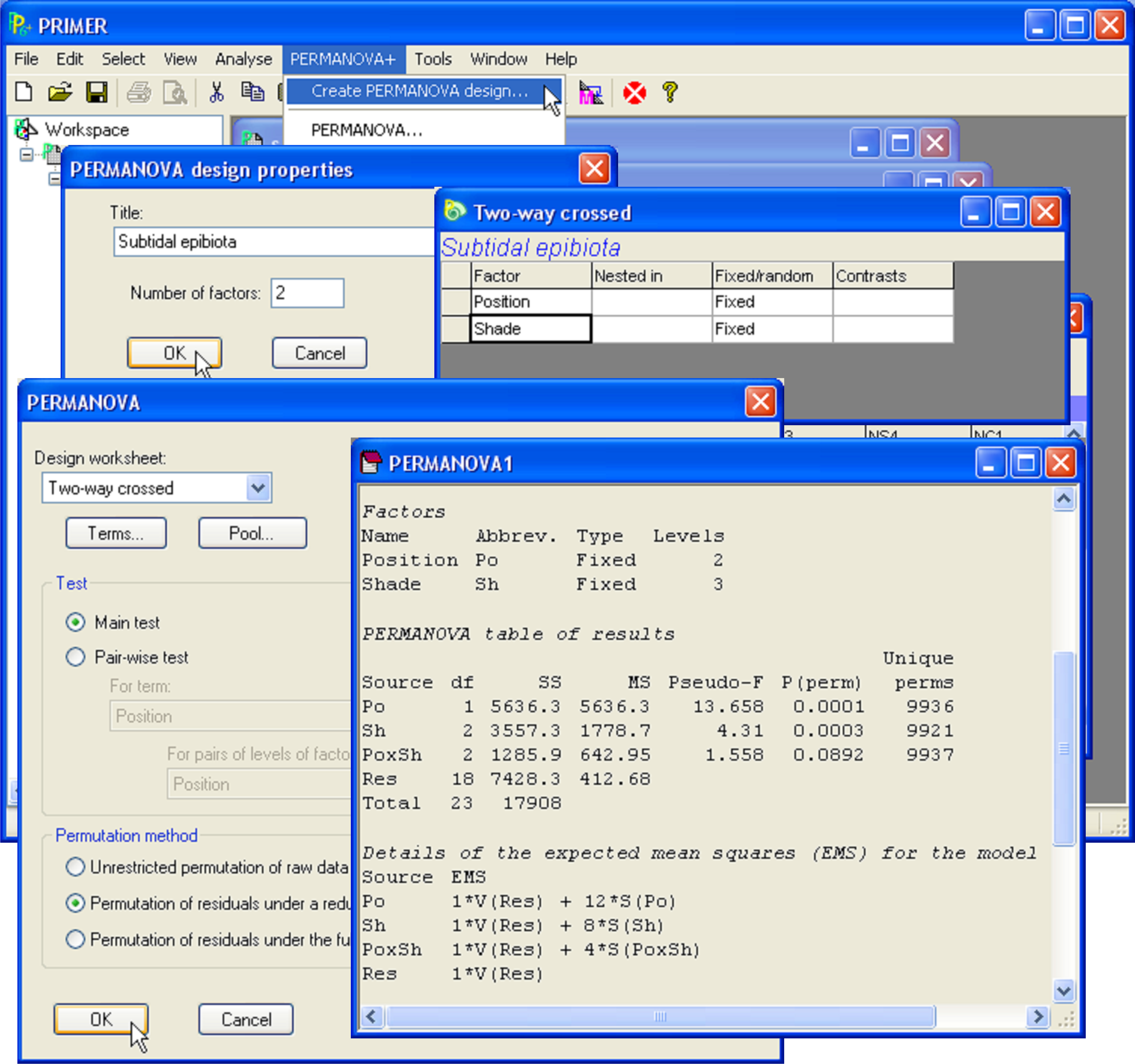 Fig. 1.15. PERMANOVA analysis of the two-way crossed design for subtidal epibiota.
Analysis by PERMANOVA proceeds according to the two steps previously outlined for the one-way case: (i) create the design file and (ii) run the PERMANOVA routine. For the first step, choose PERMANOVA+ > Create PERMANOVA design > (Title: Subtidal epibiota) > (Number of factors: 2). The design file will begin by showing 2 blank rows. Double click in the first cell of each row and select the name of each factor in turn: Position in row 1 and Shade in row 2. Choose Fixed for both of the factors in column 3 and leave columns 2 and 4 of the design file blank (Fig. 1.15). Choose File > Rename Design and rename the design file Two-way crossed, for reference. Save the workspace as sub.pwk.
Unlike the PERMANOVA routine available in DOS, it is not necessary for the order of the factors in the design file to match the order in which the factors happen to appear in the data file. PERMANOVA+ for PRIMER uses label matching to identify factors and their levels and so the order of the factors with respect to one another as they are designated within either the data worksheet or the resemblance matrix has no consequence for the analysis. However, the order of the terms in the design file does have a consequence: by default the factors are fit in the order in which they are listed in the design file. For balanced experimental designs (like this one), changing the order of terms in the model has no effect on the results anyway22. The order will matter, however, for unbalanced designs or designs with covariables if Type I sums of squares are used (see the section on Unbalanced designs).
Next, with the resemblance matrix highlighted, choose PERMANOVA+ > PERMANOVA > (Design worksheet: Two-way crossed) & (Test $\bullet$Main test) & (Sums of Squares $\bullet$Type III (partial)) & (Permutation method $\bullet$Permutation of residuals under a reduced model) & (Num. permutations: 9999). This is a more complex experimental design than the one-way case (indeed, most experimental designs involve more than one factor), so here we shall use the default method of permutation of residuals under a reduced model (see Methods of permutation for more details).
The results (Fig. 1.15) indicate that there is no statistically significant interaction in the effects of Position and Shade on variability in these assemblages, although the P-value is not large (P = 0.09). Each of the main factors do appear, however, to have strong effects (P < 0.001 for each test). These results are also reflected in the patterns seen in the MDS plot of the two factors, where labels are used to denote different levels of the Position factor and symbols are used to denote different levels of the Shade factor (Fig. 1.16).
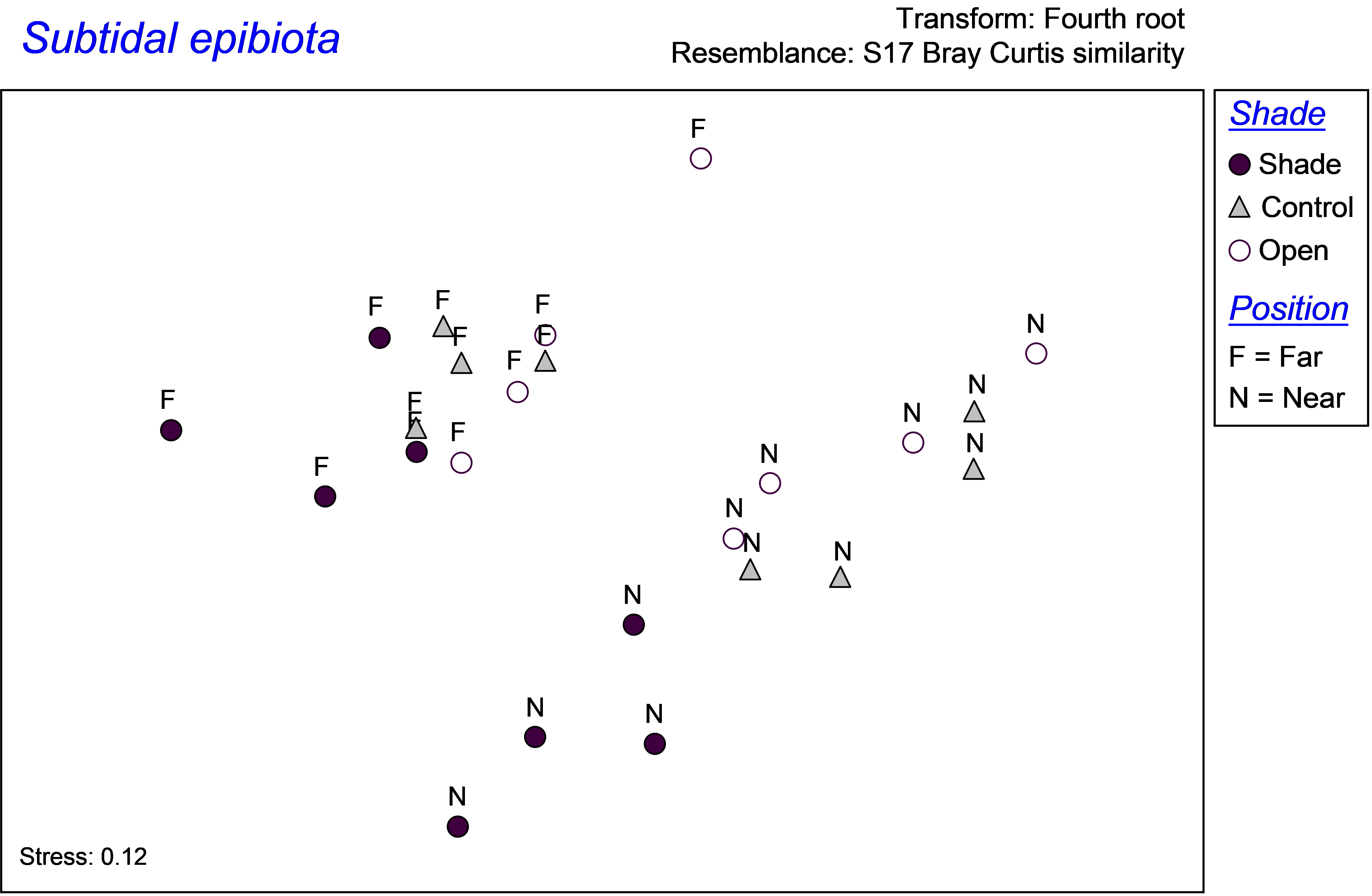 Fig. 1.16. MDS plot of subtidal epibiota with labels for the two-way crossed design.
There is a clear separation in the MDS plot between assemblages near (N) versus those far (F) from the seafloor, suggesting a strong effect of Position. There is also a tendency for the samples in the shaded treatments to occur in the lower left of the diagram, compared to those in either the procedural control or in open treatments, which occur more in the centre or upper right. Although the size of the shade effect appeared to be a bit larger for assemblages near to the seafloor than for those far from the seafloor (Fig 1.16), the direction was very similar and the test revealed no significant interaction.
21 Taxa that were present but occupied less than 1% cover were given an arbitrary value of 0.5%
22 To see this, run the PERMANOVA analysis where the first factor listed in the design file (in the first row) is Shade and the second factor in the design file is Position.