5.4 Discriminant analysis (Poor Knights Islands fish)
We will begin with an example provided by Trevor Willis and Chris Denny ( Willis & Denny (2000) ; Anderson & Willis (2003) ), examining temperate reef fish assemblages at the Poor Knights Islands, New Zealand. Divers have counted the abundances of fish belonging to each of p = 62 species in each of nine 25 m × 5 m transects at each site. Data from the transects were pooled at the site level and a number of sites around the Poor Knights Islands were sampled at each of three different times: September 1998 ($n _1$ = 15), March 1999 ($n _2$ = 21) and September 1999 ($n _3$ = 20). These times of sampling span the point in time when the Poor Knights Islands were classified as a no-take marine reserve (October 1998). Interest lies in distinguishing among the fish assemblages observed at these three different times of sampling, especially regarding any transitions between the first time of sampling (before the reserve was established) and the other two times (after).
The data are located in the file pkfish.pri in the ‘PKFish’ folder of the ‘Examples add-on’ directory. An unconstrained PCO on Bray-Curtis resemblances of log(X+1)-transformed abundances did not show a clear separation among the three groups, even though a PERMANOVA comparing the three groups was highly statistically significant (Fig. 5.3, P < 0.001). Dr Willis (quite justifiably) said: “I don’t see any differences among the groups in either a PCO or MDS plot, but the PERMANOVA test indicates strong effects. What is going on here?” Indeed, the reason for the apparent discrepancy is that the directions of the differences among groups in the multivariate space, detected by PERMANOVA, are quite different to the directions of greatest total variation across the data cloud, as shown in the PCO plot. The relatively small amount of the total variation captured by the PCO plot (the first two axes explain only 33.1%) is another indication that there is more going on in this data cloud than can be seen in two (or even three) dimensions102.
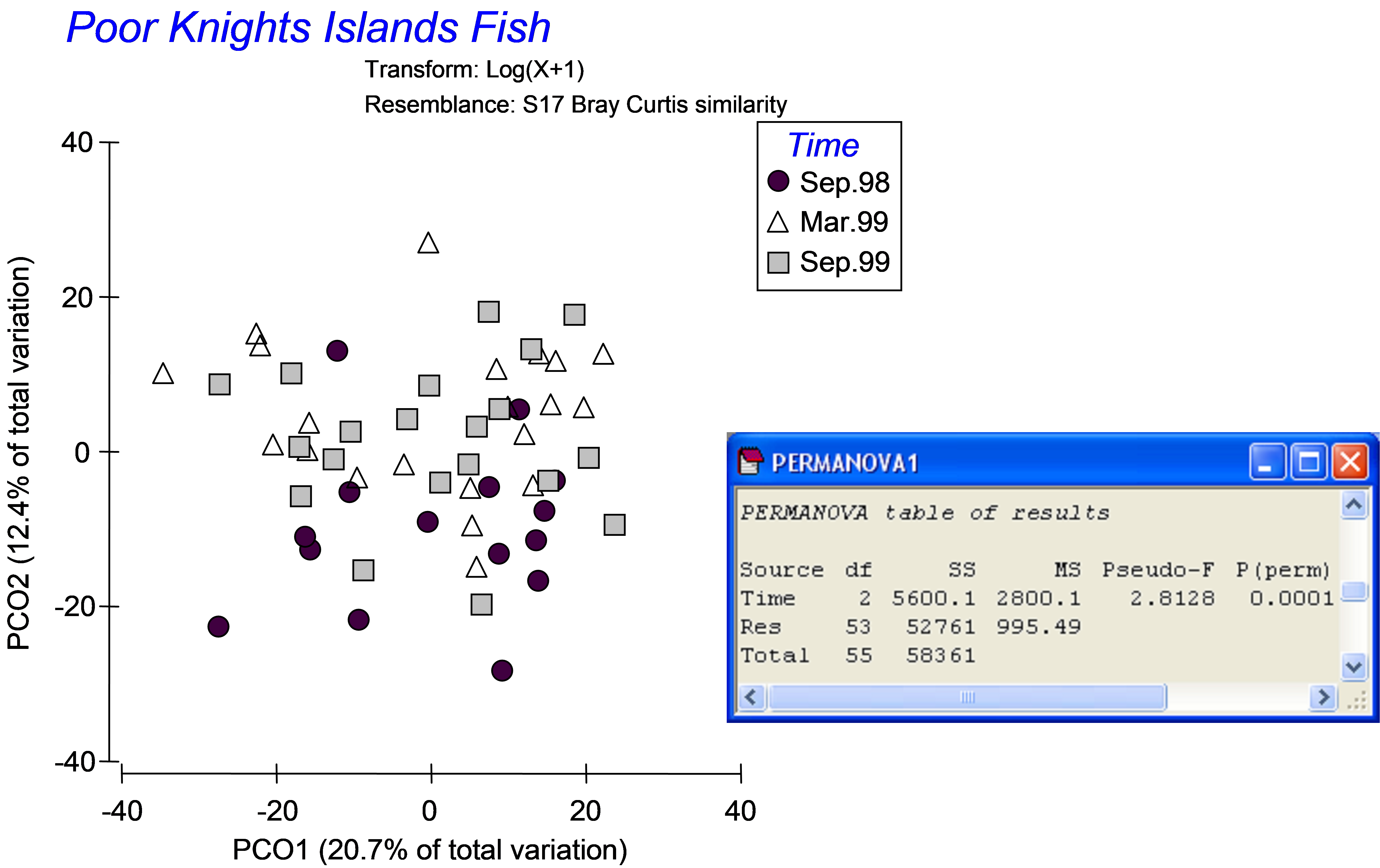
Fig. 5.3. PCO ordination and one-way PERMANOVA of fish data from the Poor Knights Islands.
To characterise these three groups of samples, to visualise the differences among them and to assess just how distinct these groups are from one another in the multivariate space, a CAP analysis can be done (Fig. 5.4). From the Bray-Curtis resemblance matrix calculated from log(X+1)-transformed data, choose PERMANOVA+ > CAP > (Analyse against •Groups in factor) & (Factor for groups or new samples: Time) & (Diagnostics $\checkmark$Do diagnostics), then click ‘OK’.
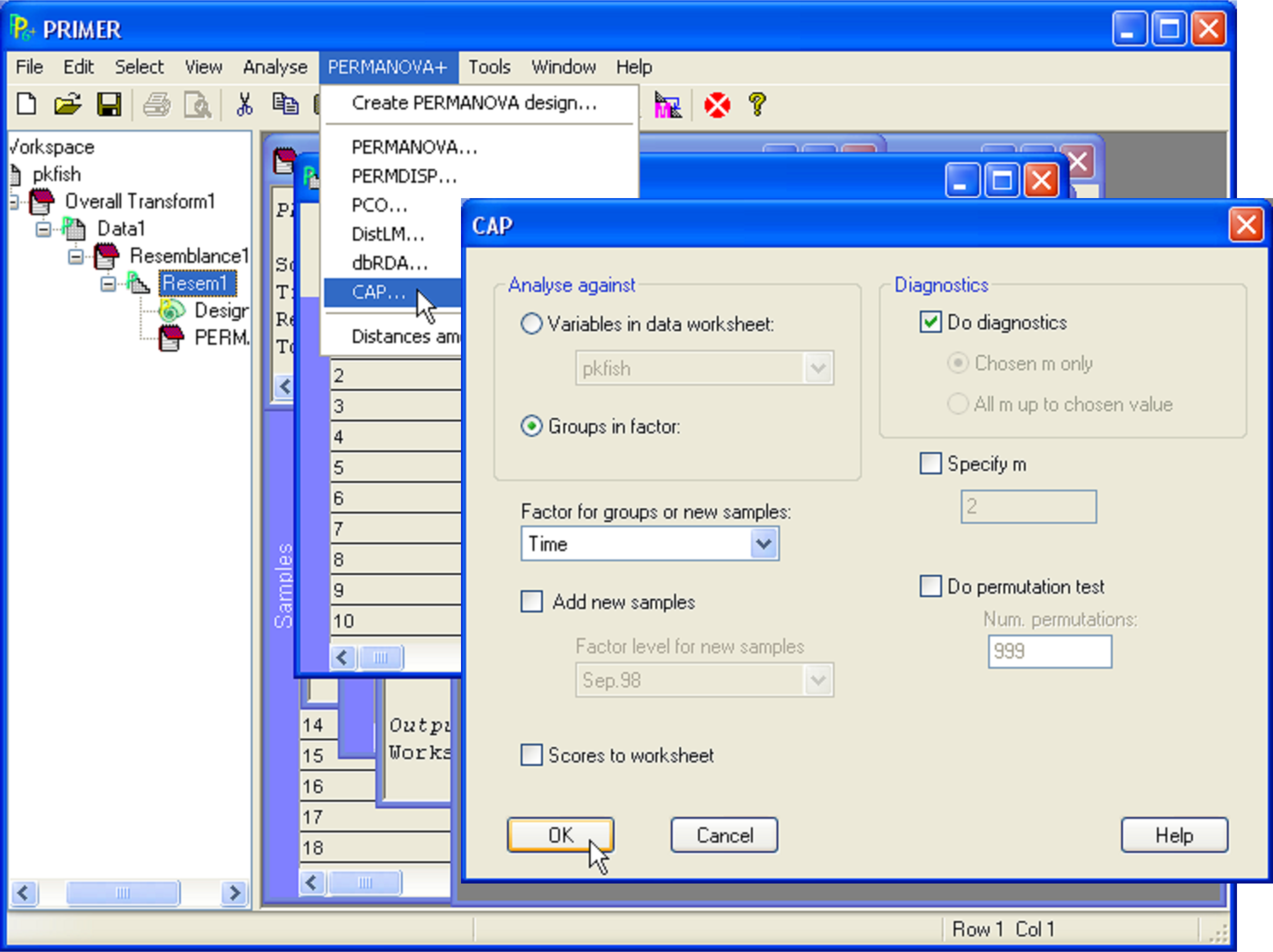 Fig. 5.4. Dialog for the CAP analysis of fish data from the Poor Knights Islands.
The resulting constrained CAP plot (Fig. 5.5) is very different from the unconstrained PCO plot (Fig. 5.3). The constrained analysis shows that the three groups of samples (fish assemblages at three different times) are indeed distinguishable from one another. The number of CAP axes produced is s = min(m, q, (N – 1)) = 2, because in this case, q = (g – 1) = 2; only 2 axes are needed to distinguish among three groups. The sizes of each of these first two canonical correlations are reasonably large: $\delta _1$ = 0.78 and $\delta _2$ = 0.69 (Fig. 5.5). These canonical correlations indicate the strength of the association between the multivariate data cloud and the hypothesis of group differences. For these data, the first canonical axis separates the fish assemblages sampled in September 1998 (on the right) from those sampled in March of 1999 (on the left), while the second canonical axis separates fish assemblages sampled in September 1999 (lower) from the other two groups (upper). Also reported in the output file is the choice for the number of orthonormal PCO axes that were used for the CAP analysis: here, m = 7. If this value is not chosen by the user, then the CAP routine itself will make a choice, based on appropriate diagnostics (see the section Diagnostics).
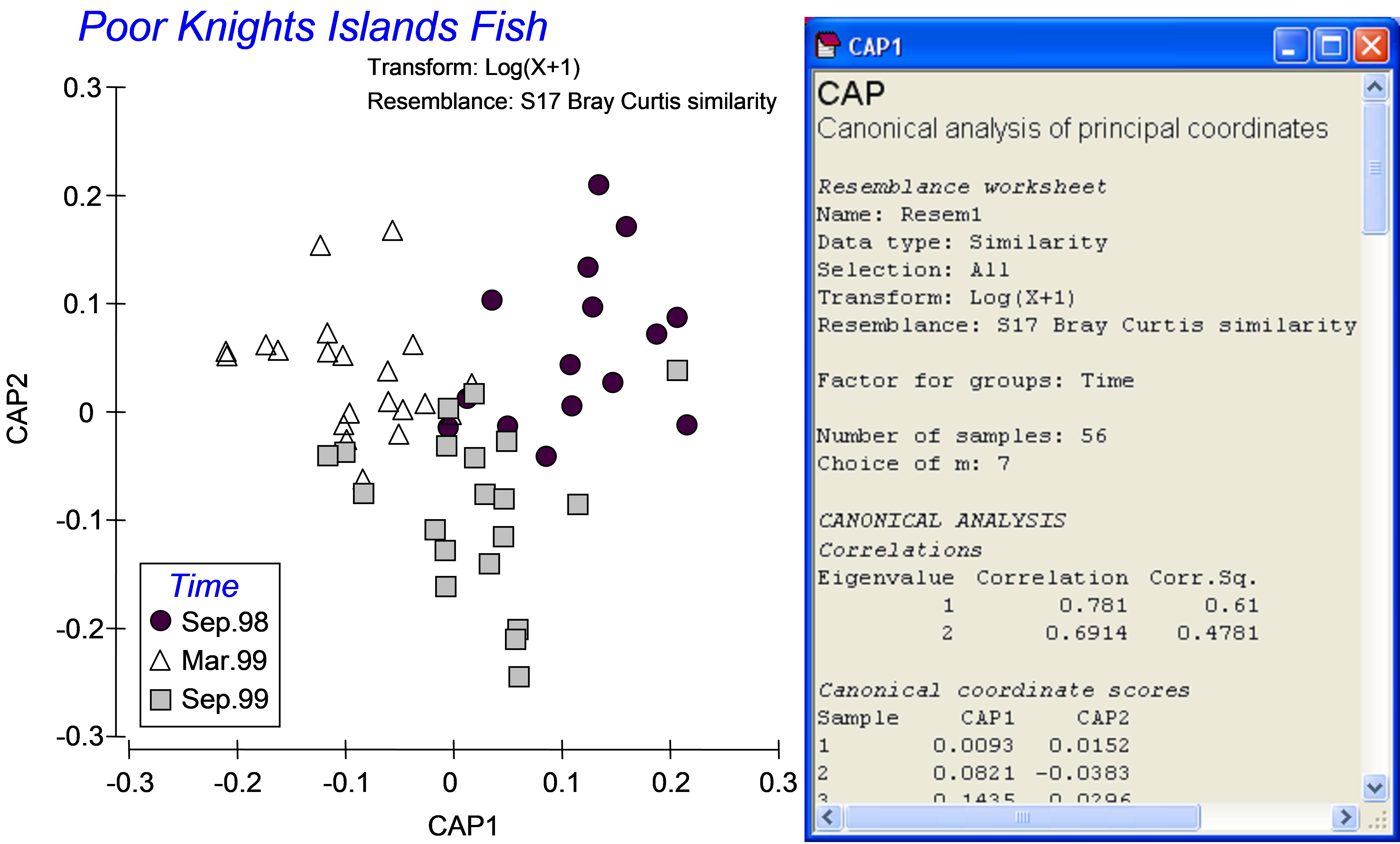 Fig. 5.5. Constrained ordination and part of the output file from the CAP analysis of fish data from the Poor Knights Islands.
A natural question to ask is which fish species characterise the differences among groups found by the CAP analysis? A simplistic approach to answer this is to superimpose vectors corresponding to Pearson (or Spearman rank) correlations of individual species with the resulting CAP axes. Although such an approach is necessarily post hoc, it is quite a reasonable approach in the case of a discriminant-type CAP analysis. The CAP axes have been expressly drawn to separate groups as well as possible, so indeed any variables which show either an increasing or decreasing relationship with these CAP axes will be quite likely to be the ones that are more-or-less responsible for observed differences among the groups.
From the CAP plot, choose Graph > Special > (Vectors •Worksheet variables: pkfish > Correlation type: Spearman ), then click on the ‘Select’ button and in the ‘Select Vectors’ dialog, choose •Correlation > 0.3 and click ‘OK’. Note that you can choose any cut-off here that seems reasonable for the data at hand. The default is to include vectors for variables having lengths of at least 0.2, but it is up to the user to decide what might be appropriate here. Note also that these correlations are for exploratory purposes only and are not intended to be used for hypothesis-testing. For example, it is clearly not appropriate to formally test the significance of correlations between individual species and CAP axes that have been derived from resemblances calculated using those very same species; this is circular logic! For more detailed information on how these vectors are drawn, see the section Vector overlays in chapter 3.
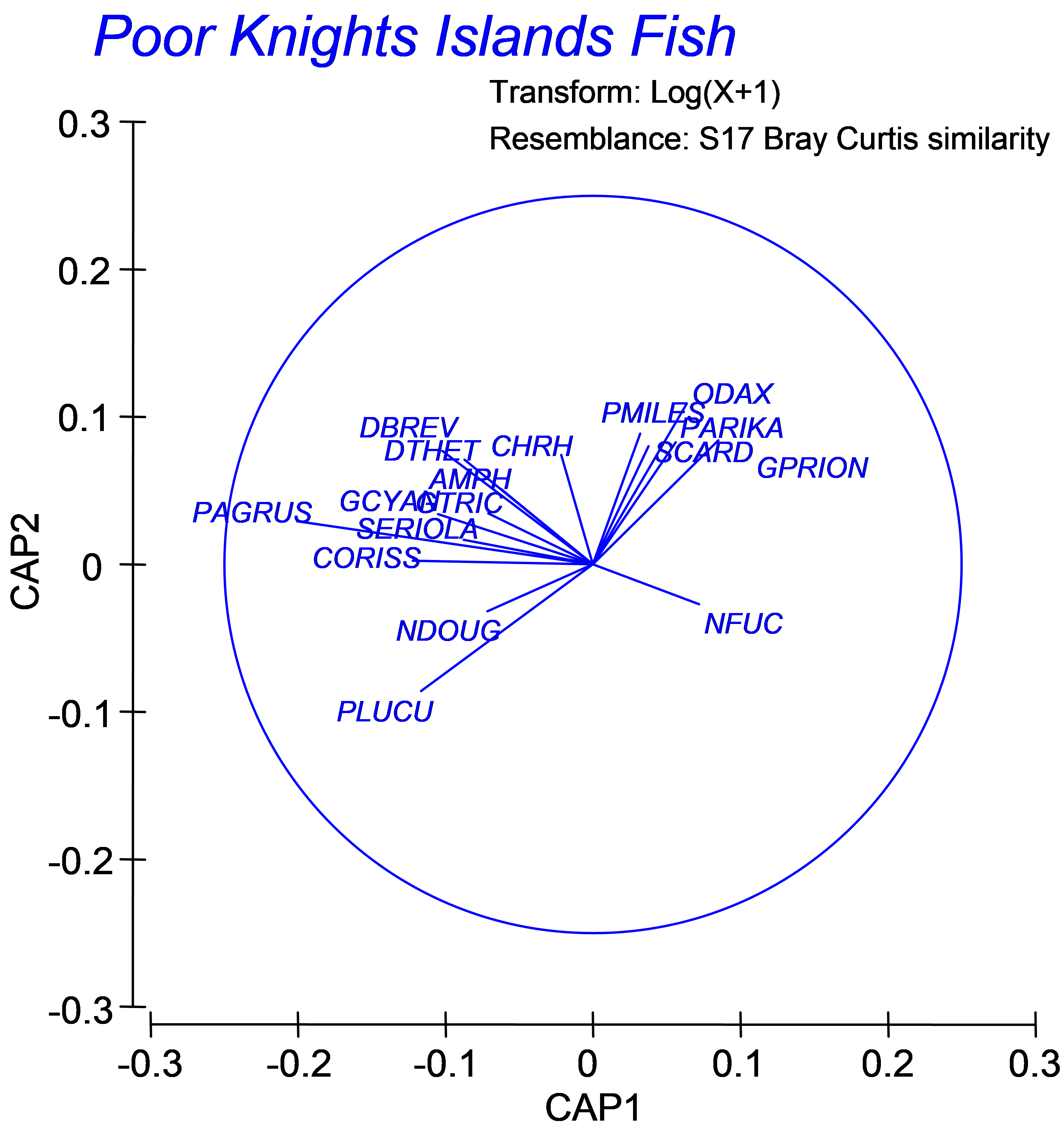 Fig. 5.6. Vector overlay of Spearman rank correlations of individual fish species with the CAP axes (restricted to those having lengths > 0.30).
For the fish assemblages from the Poor Knights (Fig. 5.6), we can see that some species apparently increased in abundance after the establishment of the marine reserve, such as the snapper Pagrus auratus (‘PAGRUS’) and the kingfish Seriola lalandi (‘SERIOLA’), which are both targeted by recreational and commercial fishing, and the stingrays Dasyatis thetidis and D. brevicaudata (‘DTHET’, ‘DBREV’). Vectors for these species point toward the upper left of the diagram in Fig. 5.6 indicating that these species were more abundant, on average, in the March 1999 samples (the group located in that part of the diagram, see Fig. 5.5). Some species, however, were more abundant before the reserve was established, including leatherjackets Parika scaber (‘PARIKA’) and the (herbivorous) butterfish Odax pullus (‘ODAX’). These results lead to new ecological hypotheses that might be investigated by targeted future observational studies or experiments.
102 Similar indications were apparent using MDS. A two-dimensional MDS of these data does not show clear differences among the groups, but has high stress (0.25). The 3-d solution (with stress also quite high at 0.18) does not show any clear differences among these three groups either, though ANOSIM, like PERMANOVA, gives clear significance to the groups (but with a low R of 0.13).