5.2 Rationale (Flea-beetles)

In some cases, we may know that there are differences among some pre-defined groups (for example, after performing a cluster analysis, or after obtaining a significant result in PERMANOVA), and our interest is not so much in testing for group differences as it is in characterising those differences. With CAP, the central question one asks is: can I find an axis through the multivariate cloud of points that is best at separating the groups? The motivation for the CAP routine arose from the realisation that sometimes there are real differences among a priori groups in multivariate space that cannot be easily seen in an unconstrained ordination (such as a PCA, PCO or MDS plot). This happens primarily when the direction through the data cloud that distinguishes the groups from one another is fundamentally different from the direction of greatest total variation across the data cloud.

For example, suppose we have two groups of samples in a two-dimensional space, as shown in Fig. 5.1. These data consist of two morphometric measurements (the distance of the transverse groove from the posterior border of the prothorax, in microns, and the length of the elytra, in 0.01 mm) on two species of flea-beetle: Haltica oleracea (19 individuals) and H. carduorum (20 individuals). For simplicity in what follows, both variables were normalised. The data are due to Lubischew (1962) , appeared in Table 6.1 of Seber (1984) and (along with 2 other morphometric variables) can be found in the file flea.pri in the ‘FleaBeet’ folder of the ‘Examples add-on’ directory.

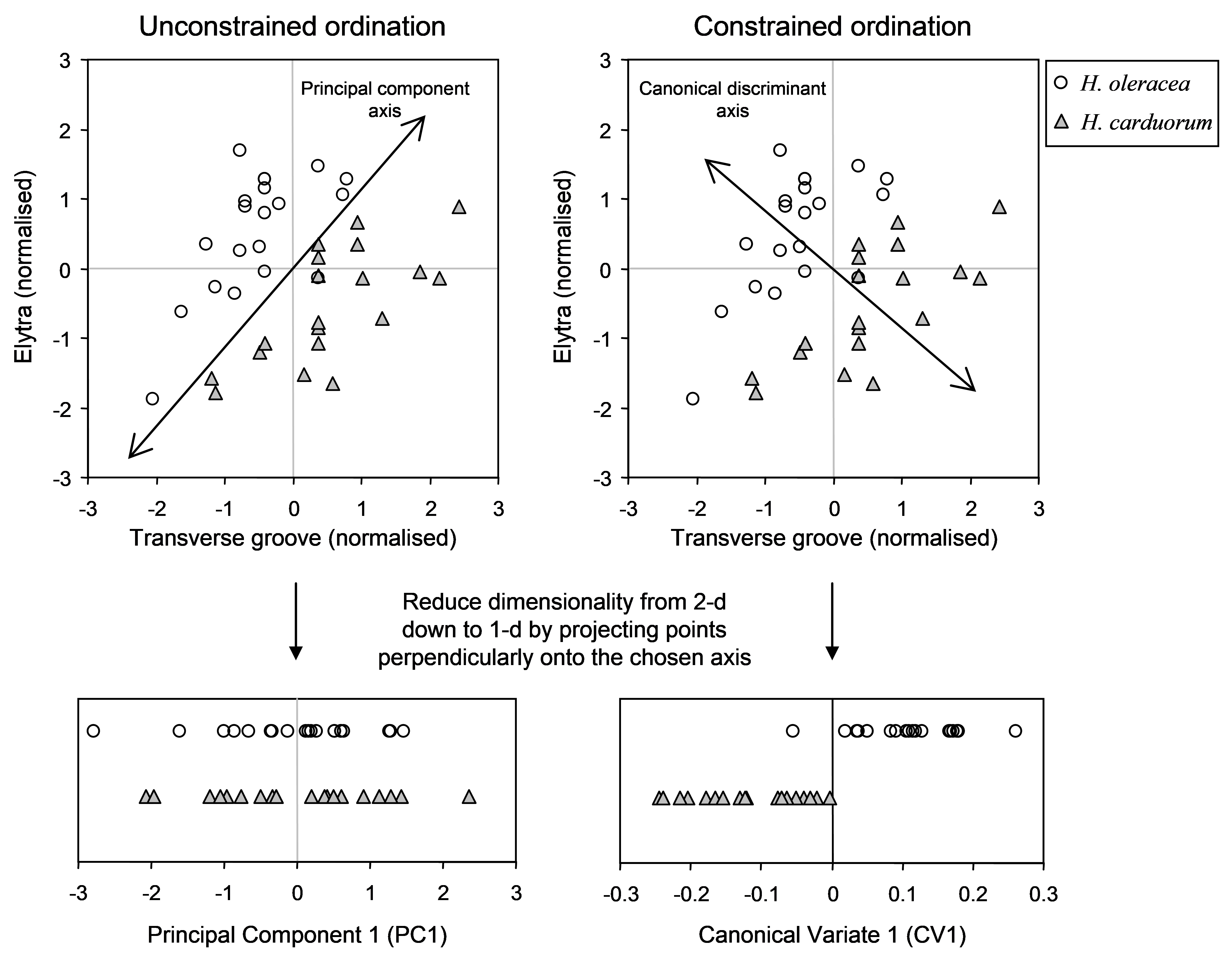Fig. 5.1. Schematic diagram showing ordinations from two dimensions (a bivariate system) down to one dimension for two groups of samples using either an unconstrained approach (on the left, maximising total variation) or a constrained canonical approach (on the right, maximising separation of the two groups).

Clearly there is a difference in the location of these two data clouds (corresponding to the two species) when we view the scatter plot of the two normalised variables (Fig. 5.1). Imagine for a moment, however, that we cannot see two dimensions, but can only see one. If we were to draw an axis through this cloud of points in such a way that maximises total variation (i.e., a principal component), then, by projecting the samples onto that axis, we would get a mixture of samples from the two groups along the single dimension, as shown on the left-hand side of Fig. 5.1. If patterns along this single dimension were all we could see, we would not suppose there was any difference between these two groups.

Next, suppose that, instead, we were to consider drawing an ordination that utilises our hypothesis of the existence of two groups of samples in some way. Suppose we were to draw an axis through this cloud of points in such a way that maximises the group differences. That is, we shall find an axis that is best at separating the groups. For this example, the direction of this axis is clearly quite different from the one that maximises total overall variation. Projecting the points onto this new axis shows, in the reduced space of one dimension, that there is indeed a clear separation of these two groups in the higher-dimensional space, even though this was not clear in the one-dimensional (unconstrained) ordination that was done in the absence of any hypothesis (Fig. 5.1).

Note that the cloud of points has not changed at all, but our view of that data cloud has changed dramatically, because our criterion for drawing the ordination axis has changed. We might liken this to visiting a city for the first time and deciding which avenue we wish to stroll down in order to observe that city. Clearly, our choice here is going to have consequences regarding what kind of “view” we will get of that city. If we choose to travel in an east-west direction, we will see certain aspects of the buildings, parks, landmarks and faces of the city. If we choose a different direction (axis) to travel, however, we will likely see something very different, and maybe get a quite different impression of what that city is like. Tall buildings might obscure certain landmarks or features from us when viewed from certain directions, and so on. Once again, the city itself (like points in a multi-dimensional space) has not really changed, but our view of it can depend on our choice regarding which direction we will travel through it.

More generally, it is clear how this kind of phenomenon can also occur in a higher-dimensional context and on the basis of some other resemblance measure (rather than the 2-d Euclidean space shown in Fig. 5.1). That is, we may not be able to see group differences in two or three dimensions in an MDS or PCO plot (both of these are unconstrained ordination methods), but it may well be possible to discriminate among groups along some other dimension or direction through the multivariate data cloud. CAP is designed precisely to do this in the multivariate space of the resemblance measure chosen.

The other primary motivation for using CAP is as a tool for classification or prediction. That is, once a CAP model has been developed, it can be used to classify new points into existing groups. For example, suppose I have classified individual fish into one of three species on the basis of a suite of morphometric measures. Given a new fish that has values for each of these same measures, I can allocate or classify that fish into one of the groups, using the CAP routine. Similarly, suppose I have done a cluster analysis of species abundance data on the basis of the Bray-Curtis resemblance measure and have identified that multivariate samples occur in four different distinct communities. If I have a new sample, I might wish to know – in which of these four communities does this new sample belong? The CAP routine can be used to make this prediction, given the resemblances between the new sample and the existing ones.

Another sense in which CAP can be used for prediction is in the context of canonical correlation. Here, the criterion being used for the ordination is to find an axis that has the strongest relationship with one (or more) continuous variables (as opposed to groups). One can consider this a bit like putting the DISTLM approach rather on its head. The DISTLM routine asks: how much variability in the multivariate data cloud is explained by variable X? In contrast, the CAP routine asks: how well can I predict positions along the axis of X using the multivariate data cloud? So, the essential difference between these two approaches is in the role of these two sets of variables in the analysis. DISTLM treats the multivariate data as a response data cloud, whereas in CAP they are considered rather like predictors instead. Thus, for example, I may use CAP to relate multivariate species data to some environmental variable or gradient (altitude, depth, percentage mud, etc.). I may then place a new point into this space and predict its position along the gradient of interest, given only its resemblances with the existing samples.