1.31 Split-plot designs (Woodstock plants)
Another special case of a design lacking appropriate replication is known as a split-plot design. These designs usually arise in an agricultural context, where the experimenter has applied the treatment levels for a factor (say, factor A) randomly to whole plots (usually within blocks of some kind) at a large scale, but then, within each of these whole plots, treatments for another factor (say, factor B) are applied randomly to smaller units. Thus, the whole plots are each “split” into smaller units. Although there are variations on this theme, the traditional split-plot design lacks replicates of the whole plots at the larger spatial scale (i.e., it is a randomised block design for factor A, with whole plots acting as the ‘error’). There is also commonly a lack of replication at the smaller spatial scale (i.e., the number of levels of factor B is equal to the number of sample units within each whole plot and these levels are allocated randomly and separately within each whole plot).
A proposed rationale for using a split-plot design is that factors may occur naturally at different scales (e.g., Mead (1988) ). Another proposed rationale is that one may already know that factor A has important effects, and one may be willing to sacrifice information on factor A to get more precise results for factor B and the interaction A×B. Although neither of these actually provides a solid argument for ignoring the need for appropriate replication in experiments, split-plot designs do still occur from time to time in biological research and can be analysed (after some thought and with care) using PERMANOVA. For more information regarding the assumptions and potential disadvantages of split-plot designs, see Mead (1988) and Underwood (1997) .
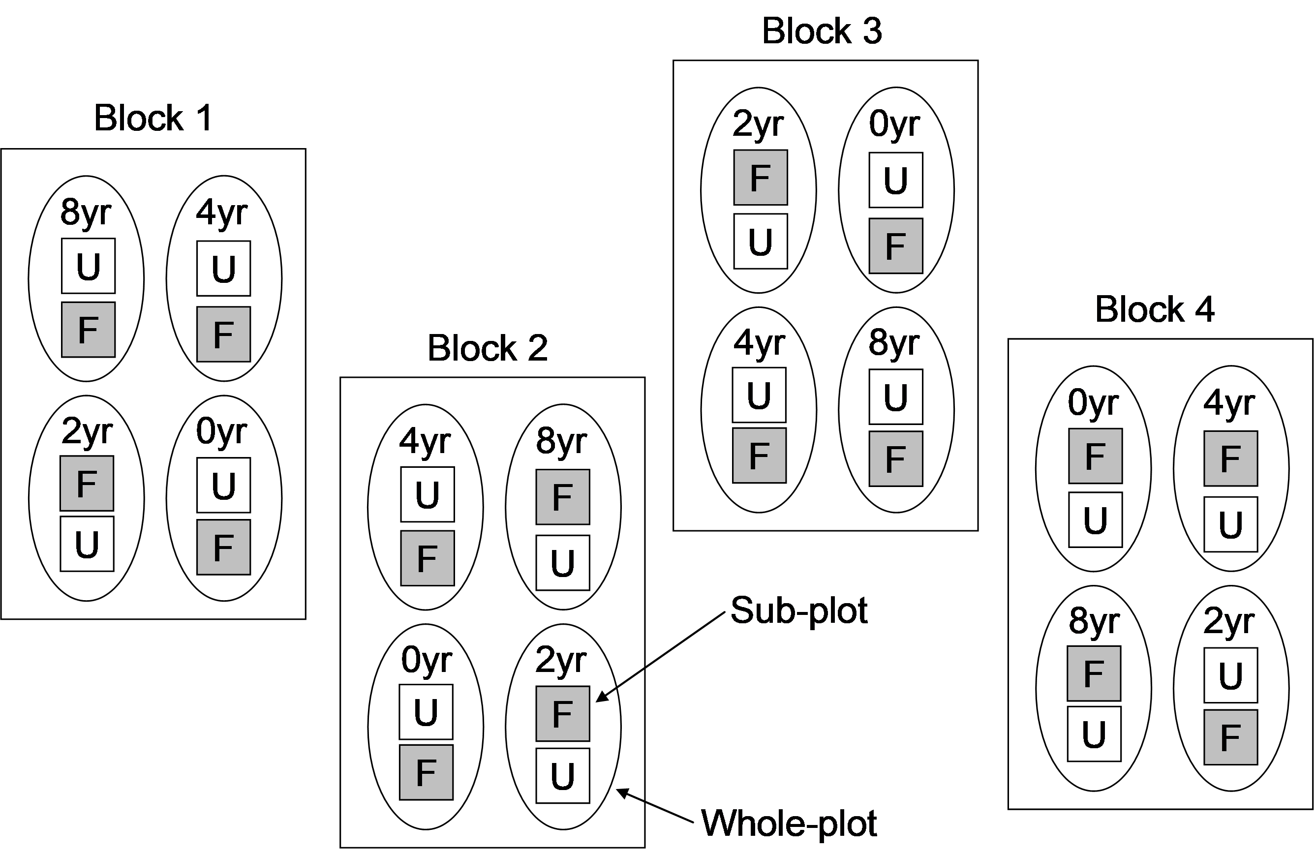
Fig. 1.35. Schematic diagram of the Woodstock split-plot design examining the potential effects of fire frequency (no burning, burning every 2 years, every 4 years or every 8 years) and the effect of grazers (by fencing some sub-plots (F), while leaving others unfenced (U)) on plant assemblages.
To analyse a split-plot design in PERMANOVA, effectively two analyses must be done: one at the ‘whole-plot’ level and one at the ‘sub-plot’ level. Results of these two analyses can then be combined to form the traditional partitioning that is usually presented for such designs. An example of a split-plot design is provided by a study of the effect of fire disturbance and fencing (to exclude grazers) on the composition of plant assemblages on the central western slopes of New South Wales in south-eastern Australia ( Prober, Thiele & Hunt (2007) ). The experimental design (shown schematically in Fig. 1.35) included the following factors:
Blocks: (random with r = 4 levels).
Factor A: Fire frequency (fixed with a = 4 levels: 0 yrs, 2 yrs, 4 yrs or 8 yrs).
Whole-plots: (random and nested within Blocks and Fire frequency, unreplicated).
Factor B: Fencing (fixed with b = 2 levels: fenced and unfenced).
Sub-plots: (random and nested within all of the above, unreplicated).
The two fencing treatments were randomly allocated to two sub-plots (measuring 5 m × 5 m) within each fire treatment (whole plots) and there is one of each fire treatment (4 whole plots) randomised within each block. Relative abundances (cover) of higher plant species within each sub-plot were estimated using a point-intercept technique (an 8 mm dowel placed vertically at each of 50 points on a grid across each plot). Although the design was set up at each of two locations (Woodstock and Monteagle) and data were obtained over a number of years ( Prober, Thiele & Hunt (2007) ), we consider here only data from the Woodstock location collected in 2003. We also will exclude two species: Poa sieberiana and Themeda australis, the dominant grasses, from the analysis. These have already been analysed separately in detail ( Prober, Thiele & Hunt (2007) ) and our focus here instead will be on the more subtle potential responses of subsidiary forbs and exotic species.
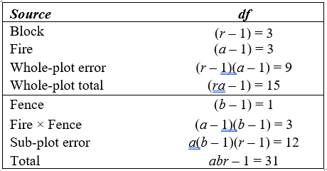
Table 1.2. Sources of variation and degrees of freedom for a traditional partitioning according to the split-plot design for the Woodstock experiment.
Partitioning for a split-plot design is traditionally done according to Table 1.2. The upper-level factors (Blocks and Fire frequency) are tested against the whole-plot error, while the lower-level factors (Fencing and the Fire × Fencing interaction term) are tested against the sub-plot error. To do this partitioning and the necessary tests using PERMANOVA, we first focus on the top-half of Table 1.2 only. This calls for a randomised block design, but where the whole plots are effectively treated as the sample units. So, first we need to obtain distances among centroids39 for the whole plots. Open the file wsk.pri (in the ‘Woodstock’ folder of the ‘Examples add-on’ directory) containing the abundances (cover measures) for p = 117 plant species. First select all of the variables except the variables numbered 50 and 63 in the dataset (‘Poa sieb’ and ‘Themaus’, respectively). Calculate a Bray-Curtis resemblance matrix after square-root transforming the selected data and choose PERMANOVA+ > Distances among centroids… > Grouping factor: WholePlot, then click ‘OK’. This yields a new matrix of Bray-Curtis resemblances among the 16 whole plots (4 fire treatments × 4 blocks). Next, run a two-way randomised block design of Block and Fire on the resemblance matrix among centroids (‘Resem2’). As there is no replication of the whole plots, you will either have to remove the ‘Block × Fire’ interaction term manually (by clicking on the ‘Terms…’ button in the PERMANOVA dialog), or let PERMANOVA do that for you. This analysis will give results for the top half (the first four terms) of the table (Fig. 1.36).
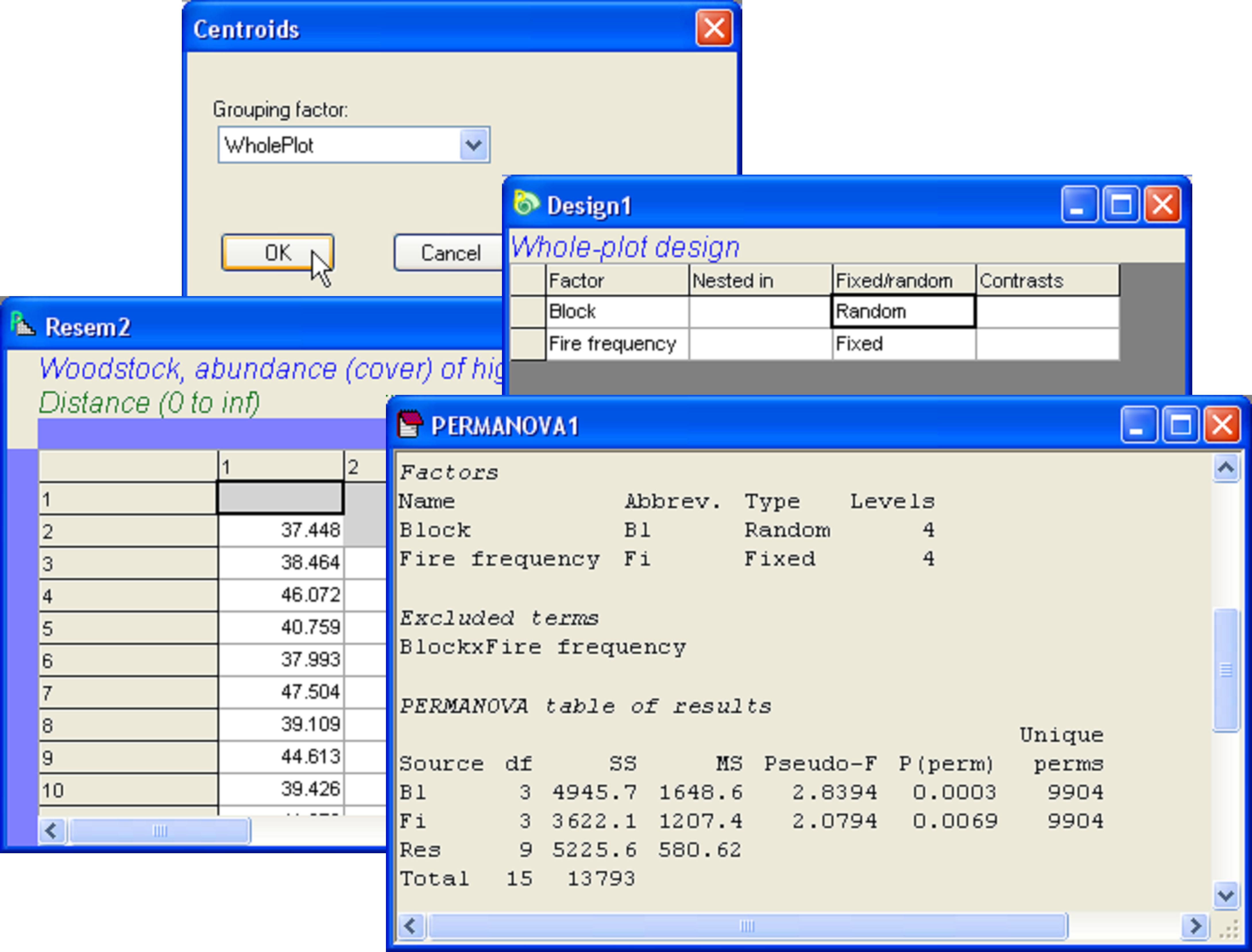
Fig. 1.36. Step one in the PERMANOVA analysis of the Woodstock split-plot design: a two-way randomised block design for whole-plots.
Now, for the lower half of the table, we will want to fit the ‘Fence’ and ‘Fire × Fence’ terms, given the whole-plots, in order to get the correct sub-plot error. Go back to the original resemblance matrix among all 32 samples (‘Resem1’) and set up a PERMANOVA design file with three factors: WholePlot, Fire frequency and Fencing (Fig. 1.37). As usual, PERMANOVA attempts to construct and fit a full model, including all interaction terms implied by the structure that is specified. In the present case, it is not possible to fit all interaction terms, because of the lack of replication. Here, it is not just the lowest level in the analysis that is unreplicated, but we also lack replication at a higher level in the design. PERMANOVA will not automatically exclude the terms that would normally be excluded from a split-plot analysis, so these must be excluded manually by clicking on the ‘Terms…’ button in the PERMANOVA dialog and choosing only those terms in the model that we wish to fit (Fig. 1.37). For this design, there are a number of terms that are purposefully excluded: namely, any interactions involving whole plots as well as the main effect of Fire. (This is on top of the fact that we have also chosen to ignore any possible interactions involving Blocks.) It is important to recognise these assumptions underlying any split-plot analysis, and the requirement to manually remove terms is a good reminder of what is going on here. Of course, if we had replicated whole-plots and replicated sub-plots, we would be in a position to analyse the whole design, including all interactions, in a single PERMANOVA analysis.
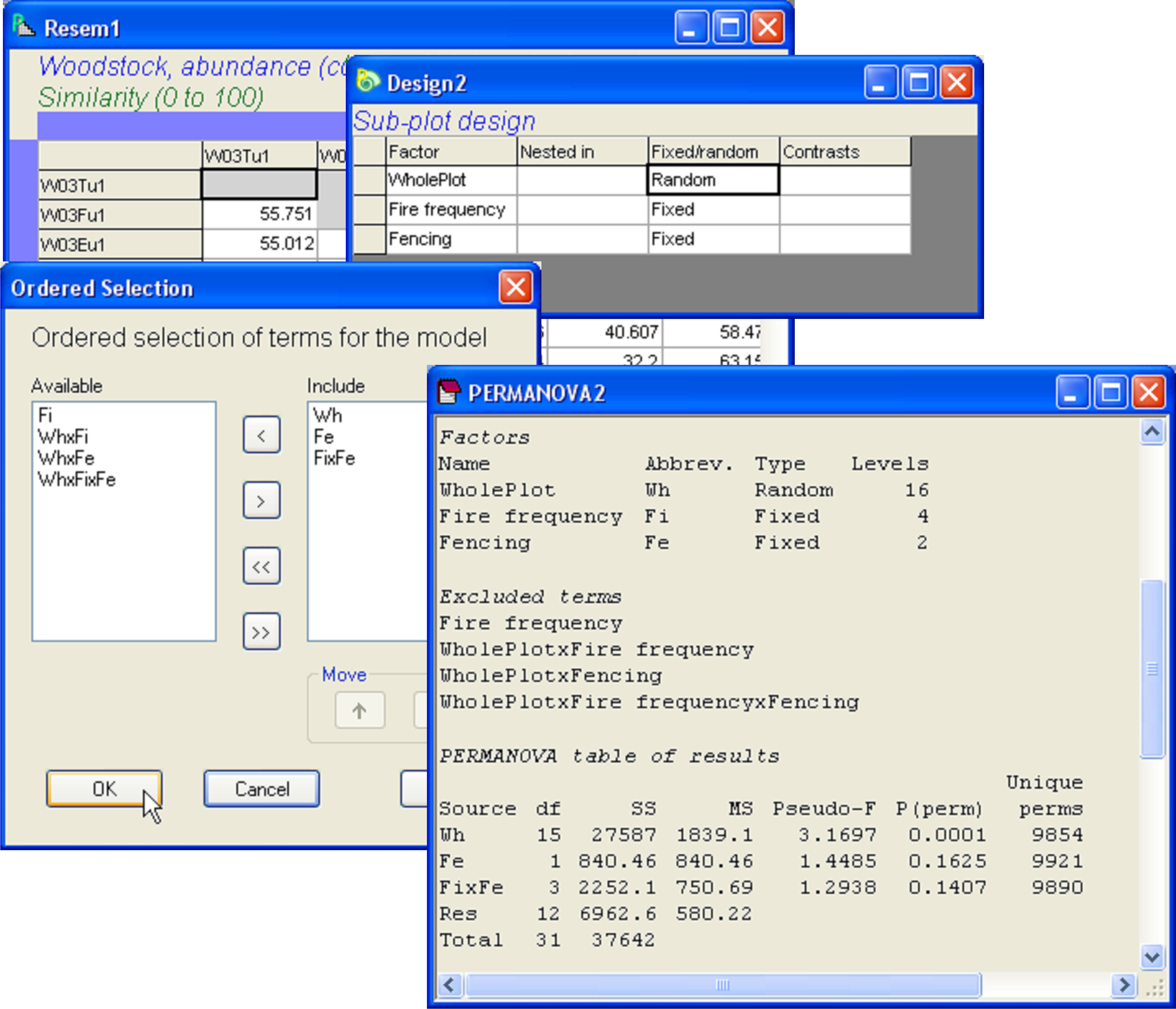
Fig. 1.37. Step two in the PERMANOVA analysis of the Woodstock split-plot design: a three-way analysis of sub-plots, excluding certain terms, but including whole-plots.
Once we have the results from both “halves” of the split-plot analysis, we can use these to construct the complete table (Table 1.3). When combining the results of more than one analysis from a single set of data, such as this, it is a good idea to check that the partitioning has been done correctly by making sure that the sum of the individual SS add up to the total SS. This is true for the present example (Table 1.3) and will be true in general, at least for a correct partitioning of any balanced design. The analysis suggests that the fencing treatments had no significant effect on these assemblages, but fire frequency did. There was no evidence that these two factors interact significantly with one another. Spatial variation among blocks and among whole plots was also substantial (see the relative sizes of components of variation in the output file).
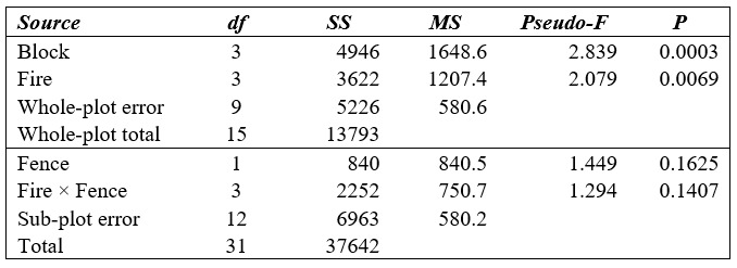
Table 1.3. Results from the PERMANOVA analysis of plant assemblages in response to fire frequency and fencing (removal of grazers) in the Woodstock split-plot experiment.
39 Importantly, these centroids are not calculated on the original data, they are calculated on the full set of PCO axes obtained from the resemblance matrix, in order to preserve the resemblance measure chosen as the basis of the analysis. For more details, see chapter 3.