10.1 Species aggregation
Fig. 10.1a repeats the multivariate ordination (nMDS) seen in Fig. 1.7 for the macrofaunal data from Frierfjord, based on 4th-root transformed species counts and Bray-Curtis similarities among the 24 samples (at 6 sites, A-E,G). The assemblage consisted of 110 taxa identified in three-quarters of the cases to the species level (the remainder, as is commonly the case, were only identified to some higher taxonomic level, e.g. Nemertines, Oligochaetes etc). Fig. 10.1b shows the same ordination plot that would have been obtained had all species-level identifications only been to the level of genus, and it is clear that the conclusions about the relationships among the 6 sites would have remained more or less identical had the identification level been that degree coarser. This is not really that surprising since many of the identified genera only contained a single species, the number of variables (taxa) reducing only from 110 species to 88 genera¶. However, the insensitivity of the multivariate analysis to the change in identification effort in this case is suggestive of more general possibilities.
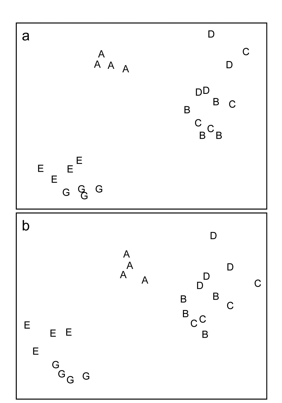
Fig. 10.1 Frierfjord macrofauna {F}. Sample MDS using Bray-Curtis similarities on $ \sqrt{} \sqrt{} $-transformed counts for a) 110 species, b) 88 genera (stress = 0.10, 0.09 respectively).
The painstaking work involved in sorting and identifying samples to the species level has resulted in community analysis for environmental impact studies being traditionally regarded as labour-intensive, time-consuming and therefore relatively expensive. One practical means of overcoming this problem might therefore be to try analysing the samples to some higher taxonomic level, such as family. If results from this coarser level are comparable to full species analysis, this means that:
a) A great deal of labour can be saved. Several groups of marine organisms are taxonomically difficult, for example (in the macrobenthos) several families of polychaetes and amphipods; as much time can be spent in separating a few of these difficult groups into species as the entire remainder of the sample, even in Northern Europe where taxonomic keys for identification are most readily available.
b) Less taxonomic expertise is needed. Many taxa really require the skills of specialists to separate them into species, and this is especially true in parts of the world where fauna is poorly described. For certain groups of marine organisms, e.g. the meiobenthos, the necessary expertise required to identify even the major taxa (nematodes and copepods) to species is lacking in most laboratories which are concerned with the monitoring of marine pollution, so that these components of the biota are rarely used in such studies, despite their many inherent advantages (see Chapter 13).
For the marine macro- and meiobenthos, aggregations of the species data to higher taxonomic levels are examined below in a few applications, and resultant data matrices subjected to several forms of statistical analysis to see how much information has been lost compared with species-level analysis. Examples are also seen in Chapter 16, where a more sophisticated methodology is given for summarising the relative effects of differing levels of taxonomic aggregation, in comparison with other decisions that need to be made about a multivariate analysis, e.g. severity of transformation and choice of resemblance measure (we defer such discussion until the needed tools have been presented in Chapters 11 and 15). Aggregation, followed by simple re-analysis, has now been looked at very widely in the marine (and non-marine) literature for a range of faunal groups.
Methods amenable to aggregation
- Multivariate methods. Although taxonomic levels higher than that of species can be used to some degree for all types of statistical analysis of community data, it is probably for multivariate methods that this is most appropriate, at least when the taxa is relatively species rich; e.g. Chapter 16 shows the high degree of structural redundancy in marine macrobenthic assemblages, with many sets of species ‘carrying the same information’, in effect, about the spatio-temporal changes which drive the community patterns. (On the other hand, it is clear that for a very limited faunal group such as, say, the freshwater fish of Australian river systems, with species numbers typically only in single figures, there is much to lose and little to gain by aggregation to higher taxa). All ordination/clustering techniques are amenable to aggregation, and there is now substantial evidence that identification only to the family level for macrobenthos, and the genus level for meiobenthos, makes very little difference to the results (see, for example, Figs. 10.2–10.6, and the results in Chapter 16). There are possibly also theoretical advantages to conducting multivariate analyses at a high taxonomic level for pollution impact studies. Natural environmental variables which also affect community structure are rarely constant in surveys designed to detect pollution effects over relatively large geographical areas. For the benthos, such ‘nuisance’ variables include water depth and sediment granulometry. However, it is a tenable hypothesis that these variables influence the fauna more by species replacement than by changes in the proportions of the major taxa present. Each major group, in its adaptive radiation, has evolved species which are suited to rather narrow ranges of natural environmental conditions, whereas anthropogenic contamination has been too recent for the evolution of suitably adapted species. Ordinations of abundance or biomass data of these major taxa are thus more likely to correlate with a contaminant gradient than are species ordinations, the latter being more complicated by the effects of natural environmental variables. In short, higher taxa may well reflect well-defined pollution gradients more closely than species.
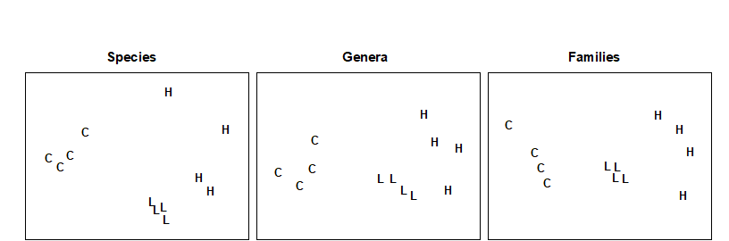
Fig. 10.2. Nutrient-enrichment experiment, Solbergstrand {N}. MDS plot of copepod abundances ($ \sqrt{} \sqrt{} $-transformed, Bray-Curtis similarities) for 4 replicates from 3 treatments; species data aggregated into genera and families (stress = 0.09, 0.09, 0.08).

Fig. 10.3. Loch Linnhe macrofauna {L}. MDS (using Bray-Curtis similarities) of samples from 11 years. Abundances are $ \sqrt{} \sqrt{} $-transformed (top) and untransformed (bottom), with 111 species (left), aggregated into 45 families (middle) and 9 phyla (right). (Reading across rows, stress = 0.09, 0.09, 0.10, 0.09, 0.09, 0.02).
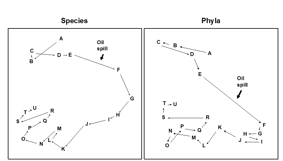
Fig. 10.4. Amoco-Cadiz oil spill {A}. MDS for macrobenthos at station ‘Pierre Noire’ in the Bay of Morlaix. Species data (left) aggregated into phyla (right). Sampling months are A:4/77, B:8/77, C:9/77, D:12/77, E:2/78, F:4/78, G:8/78, H:11/78, I:2/79, J:5/79, K:7/79, L:10/79, M:2/80, N:4/80, O:8/80, P:10/80, Q:1/81, R:4/81, S:8/81, T:11/81, U:2/82. The oil-spill was during 3/78, (stress = 0.09, 0.07).
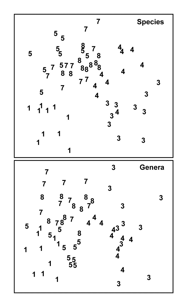
Fig. 10.5. Indonesian reef corals {I}. MDS for species (p=75) and genus (p=24) data at South Pari Island (Bray-Curtis similarities on untransformed % cover). The El Niño occurred in 1982–3. 1=1981, 3=1983 etc. (stress = 0.25).
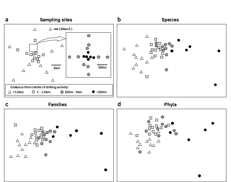
Fig. 10.6. Ekofisk oil-platform macrobenthos {E}. a) Map of station positions, indicating symbol/shading conventions for distance zones from the centre of drilling activity; b)-d) MDS for root-transformed species, family and phyla abundances (stress = 0.12, 0.11, 0.13).
-
Distributional methods. Aggregation for ABC curves is possible, and family level analyses are often identical to species level analyses (Fig. 10.7).
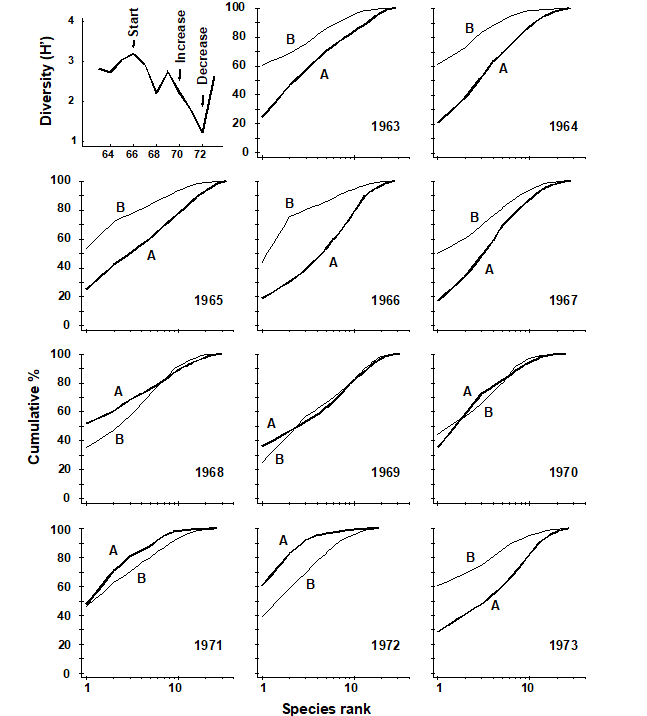
Fig. 10.7. Loch Linnhe macro¬fauna {L}. Shannon diversity (H´) and ABC plots over the 11 years, 1963 to 1973, for data aggregated to family level (c.f. Fig. 8.7). Abundance = thick line, biomass = thin line.
- Univariate methods. The concept of pollution indicator groups rather than indicator species is well-established. For example, at organically enriched sites, polychaetes of the family Capitellidae become abundant (not just Capitella capitata), as do meiobenthic nematodes of the family Oncholaimidae. The nematode copepod ratio ( Raffaelli & Mason (1981) ) is an example of a pollution index based on higher taxonomic levels. Such indices are likely to be of more general applicability than those based on species level data. Diversity indices themselves can be defined at hierarchical taxonomic levels for internal comparative purposes, although this is not commonly done in practice.
¶ This pooling of counts to any specified coarser taxonomic level (called aggregation by PRIMER) uses the Aggregate routine on the Tools menu and requires a look-up table, an aggregation file, which can consist of a much larger species set (probably in a different order), from which each variable (species) in the data matrix is allocated to a specified genus, family, order, class, etc. Such aggregation files are also of fundamental importance in computing biodiversity measures based on the taxonomic relatedness of species in each sample, see Chapter 17.