6.17 Example: Tees Bay macrofauna
The final example in this chapter is of a mixed nested and crossed design B$\times$C(A), for a total of 192 macrobenthic samples (282 species) from: A: four sub-tidal Areas of Tees Bay (Fig. 6.18, top left), with C: two Sites from each area, the same sites being returned to each September over B: 24 Years (1973-1996), part of a wider study of the Tees estuary, Warwick, Ashman, Brown et al. (2002) , {t}. Sites (C) are therefore nested in Areas (A) but crossed with Years (B). There was a further level of replication, with multiple grab samples collected but these have been averaged to give a more reliable picture of the assemblage on that occasion (the repeat grabs from a single ship stationing being considered ‘pseudo-replicates’ in time, and possibly space). The areas lie on a spatial transect (c. 5km spacing) but are probably not ordered hydrodynamically, so we shall contrast both ordered and unordered tests for A (cases 3m/3j in Table 6.4). The years are also amenable to analysis under either assumption: as it happens, there is a clear annual trend in assemblage structure over the period (seen in the right-hand plots of Fig. 6.18, for the two sites in each area averaged), but the prior expectation might have been for a more complex time signal of cycles or short-term changes and reversions, so this data will serve as an illustration of both the case of B ordered or unordered (cases 3l/3j). There being only two sites in each area, it is then irrelevant whether C is considered ordered or not; with no real replication, there can be no test for a site effect from only two sites (though there would be a test with a greater number of sites, either ordered or not, 3k/3j).
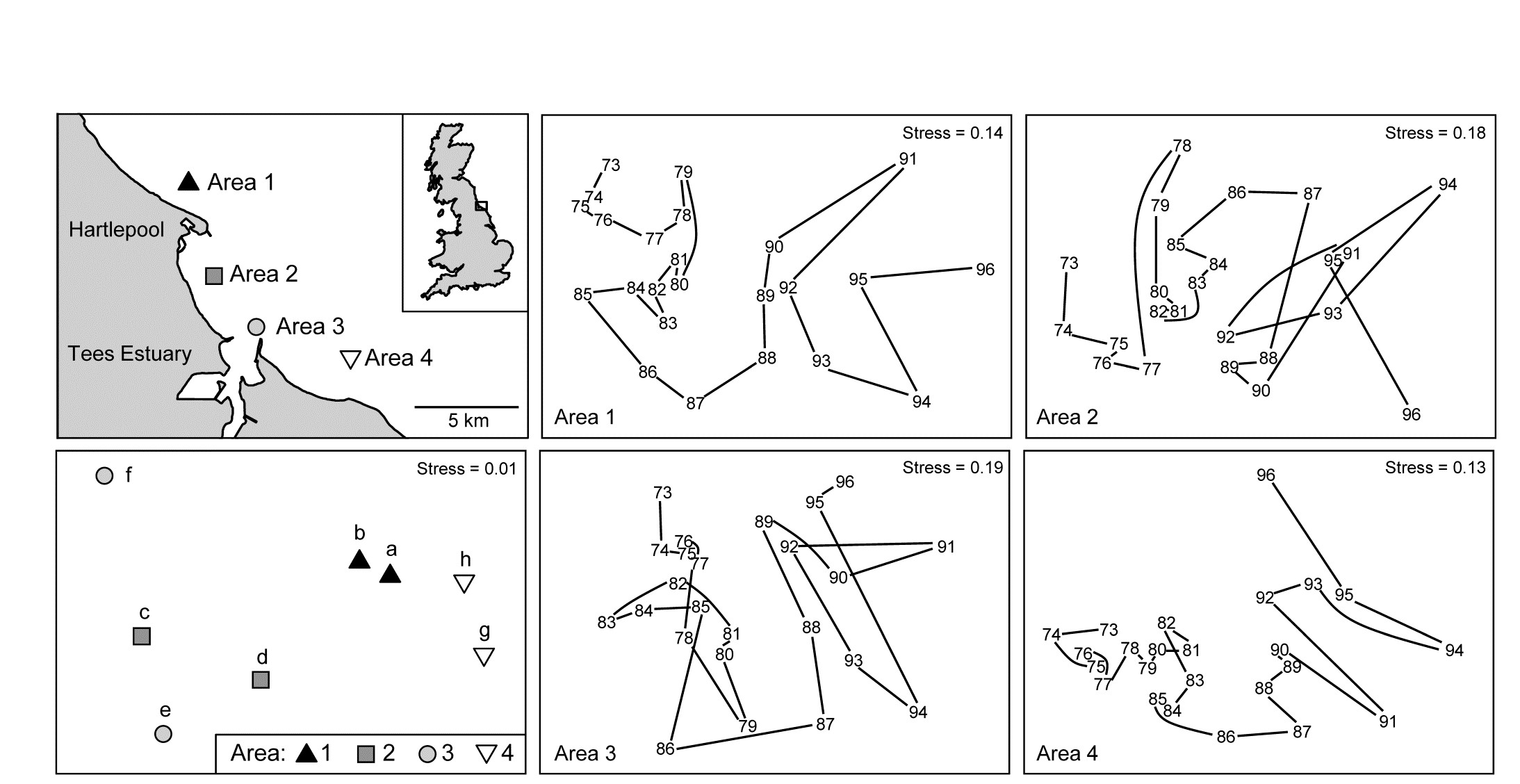
Fig. 6.18. Tees Bay macrofauna {t}. Map of four sampling areas in Tees Bay, NE England, and separate nMDS time-series plots for each area, of the macrobenthic assemblages over 24 years of September sampling; abundances were fourth-root transformed then averaged over the two sites in each area, then input to Bray-Curtis similarity calculation. Bottom left plot is the nMDS of averages of transformed abundances over the 24 time points for the two sites (a-b, c-d, e-f, g-h) in each of the four areas.
Test for Area factor (A)
The schematic below displays the construction of the ANOSIM permutation test for area (A), case 3m/3j¶.

The building blocks are the 1-way ANOSIM statistics $R$ (or $R^{Oc}$ if A is considered ordered) for a test of the 4 areas, using as replicates the 2 sites in each area, computed separately for each year. These are then averaged over the 24 years, to obtain the overall test statistic for A of $\overline{R}$ (or $\overline{R}^{Oc}$), exactly as for the usual 2-way crossed case A$\times$B met on page 6.7. The crucial difference however is in generating the null hypothesis distribution for this test statistic. Permuting the 8 sites across the 4 areas separately for each year, as the standard A$\times$B test would do, is to assume that the sites are randomly drawn afresh each year from the defined area, rather than determined only once and then revisited each year. The relevant permutation is therefore to keep the columns of this schematic table intact and shuffle the 8 whole columns randomly over the 4 areas, recalculating $\overline{R}$ (or $\overline{R}^{Oc}$) each time. There will be many fewer permutations for the A test under this B$\times$C(A) design (8!/2!2!2!2!4! =105 for the unordered case, compared with $105^{24}$) but what it loses in ‘power’ here it may make up for in improved focus when examining the time factor: subtle assemblage changes from year to year may be seen by returning to the same site(s), and these might otherwise get swamped by large spatial variability from site to site, if the latter are randomly reselected each year.
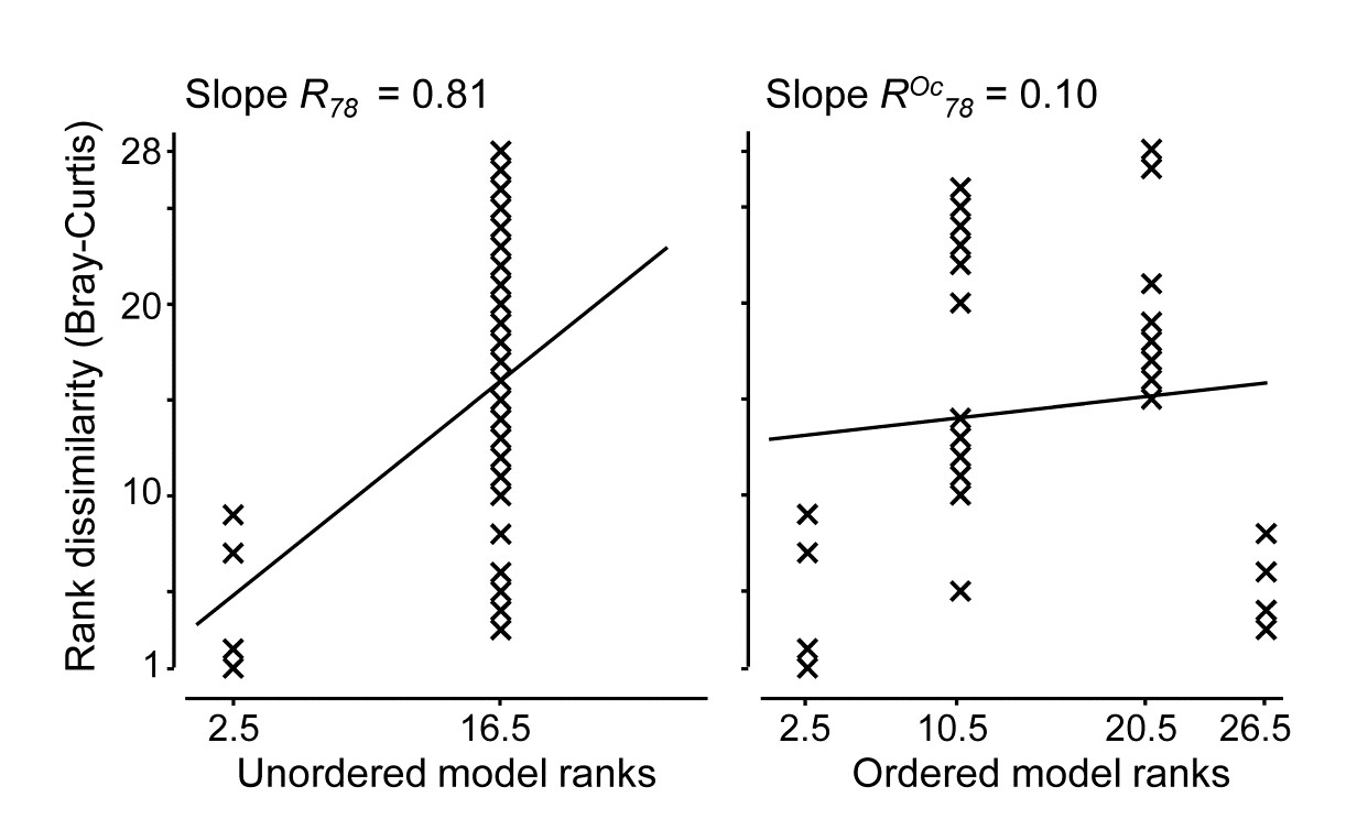
If area is considered an unordered factor, $\overline{R}= 0.60$, a high value (and the most extreme of the 105 permutations, so p = 1%); this is clearly seen in the time-averaged MDS plot for the 8 sites (Fig. 6.18, lower left). If treated as an ordered factor, the area test gives $\overline{R}^{Oc} = 0.13$, now not even significant. These two $\overline{R}$ values are directly comparable; both are slopes of a linear regression of the type seen in Fig. 6.13b, with the same y axis values but only two rather than four x axis points in the unordered case (within and among groups, as earlier explained). The MDS plot of sites in Fig. 6.18 makes clear the down side of an ordered test, based solely on the NW to SE transect of areas: here the middle two areas are within the confines of Tees Bay, their assemblages potentially influenced by the hydrodynamics or even anthropogenic discharges from the Tees estuary. Thus areas 1 and 4 are rather similar to each other but differ from areas 2 and 3. Opting for what can be a more powerful test if there is a serial pattern risks failing to detect obvious differences when they are not serial, as illustrated below for one of the 24 components of the average $\overline{R}$ and $\overline{R}^{Oc}$, namely the $R$ and $R^{Oc}$ constructions for 1978:
Test for Year factor (B)
Turning to the test for the Year factor (B), case 3l/3j in Table 6.4, the schema for construction of the test statistic in both ordered and unordered cases is now:
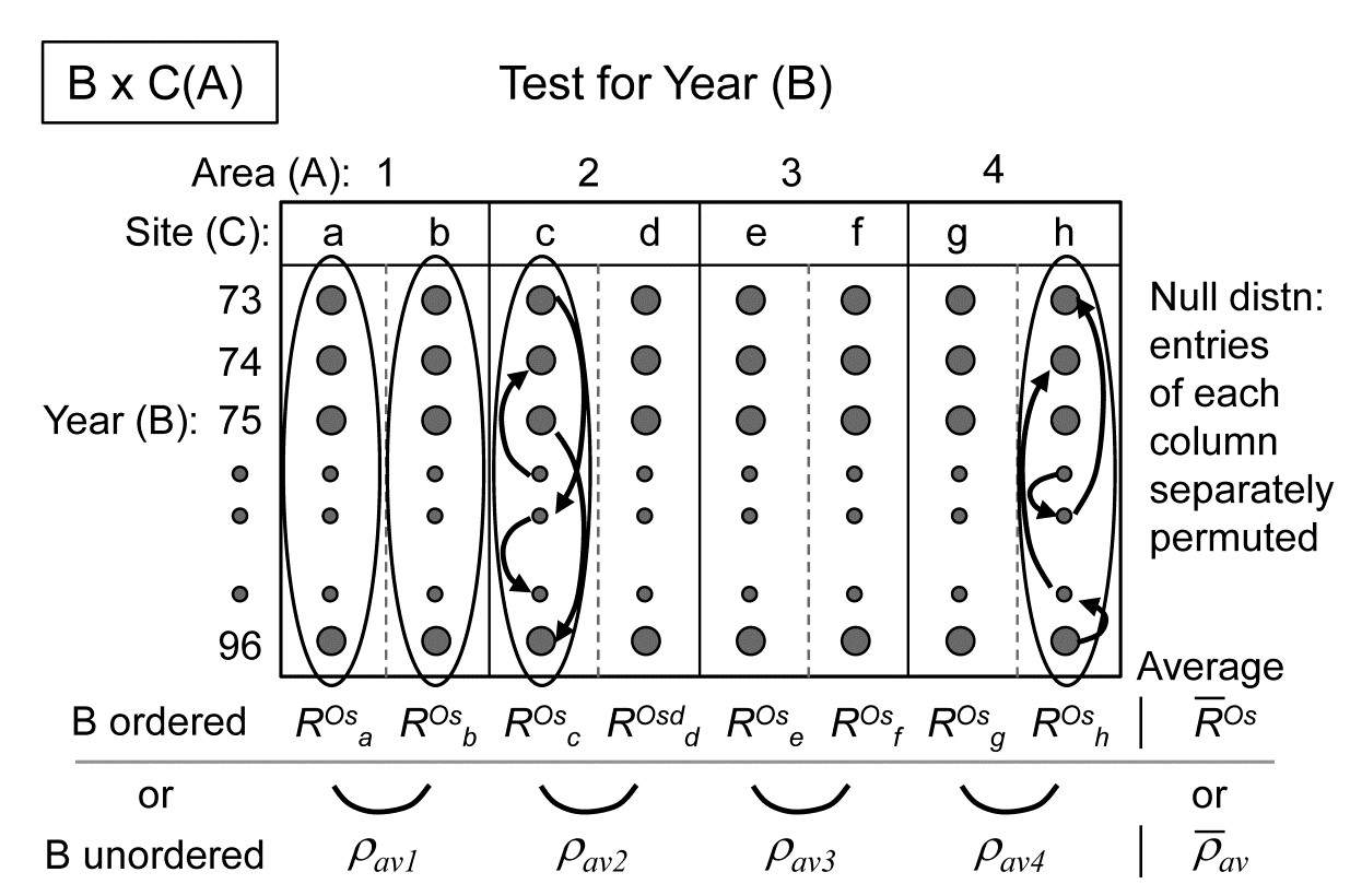
When years are considered ordered, the test reduces to the 2-way crossed layout B$\times$C (case 2d, Table 6.3) in which a 1-way ordered ANOSIM statistic without replicates ($R^{Os}$) is calculated over years, separately for each of the 8 sites, and these values averaged to give $\overline{R}^{Os}$, exactly the test for trend seen in Fig. 6.14 for the Phuket coral reef data (though there the trend was for spatial positions averaged over years, whilst here it is the opposite, of inter-annual trends averaged over sites). The appropriate permutation is the usual one of samples in each site being randomly permuted across the years (since the null hypothesis specifies that there is no year effect, at any site). As Fig. 6.18 illustrates, this will be roundly rejected, with global $\overline{R}^{Os} = 0.52$, which is significant at any fixed level, in effect, as shown by the null permutation distribution:

If it is considered unwise to test only for a time trend, rather than a more general pattern of annual changes, there is no replication which the test for B can exploit so the design falls back on an indirect test of the type introduced in Fig. 6.9: evidence of differences among years is provided by a commonality of time patterns in space. A modified test statistic is needed here to cope with the structuring of the spatial factors into a 2-way nested design of sites within areas. As shown in the above schematic diagram, a logical construction for the test statistic here is to use the matching statistic $\rho_{av}$ among the sites within each area (though in this case there is only one $\rho$ since there are only 2 sites) and then average this across the areas, to give a doubly-averaged $\overline{\rho}_ {av}$ statistic. If there are no annual differences this will, as usual, take the value zero, and the null hypothesis distribution is created by the same permutations as for the ordered test. An inter-annual effect is therefore inferred from consistency in time patterns between sites. If (as might well be thought in this context) it is more appropriate to infer consistent temporal change by noting commonality at the wider spatial scale of areas, then the sites should simply be averaged (see previous footnotes on how best to do this) to leave a 2-way A$\times$B design with both factors unordered, and the B test uses the (singly-averaged) $\rho_{av}$ statistic of Fig. 6.9.
Generally one might expect the time pattern to be less consistent as the spatial scale widens, but here, based on sites, $ \overline{\rho}_ {av} = 0.62$ and on areas, $\rho_ {av} = 0.66$, perhaps because averaging sites removes some of the variability in the sampling. Both $\rho$ statistics are again highly significant, though note that they cannot be compared with the $\overline{R}^{Os}$ value for the ordered case; the statistics are constructed differently.
Returning to the $\overline{R}^{Os}$ test for temporal trend, doubly averaging the statistics in that case, by site then area, could not actually change the previous value (0.52), though averaging sites first and performing the 2-way design on areas $\times$ years does increase the value to $\overline{R}^{Os} = 0.60$, for the same reasons of reduction in sampling ‘noise’; it is this statistic that reflects the overall trend seen in the four right-hand plots of Fig. 6.18. It would generally be of interest to ask whether the averaged $\overline{R}^{Os}$ hides a rather different trend for each area, and the individual trend values $R^{Os}$ for each area (or site) could certainly be calculated and tested. The 4 areas here give the reasonably consistent values $R^{Os}$ = 0.67, 0.54, 0.50, 0.67 respectively (all p<<0.01%), though there is perhaps a suggestion here and in the plots that the wider regional trend seen in Areas 1 and 4, and for which there is evidence from other North Sea locations (a potential result of changing hydrodynamics), is being impacted by more local changes within the Tees estuary, which will affect areas 2 and 3, within Tees Bay. This is a form of interaction between Year and Area factors and we shall see later that limited progress can be made in exploring this type of interaction non-parametrically, through the definition of second-stage MDS and tests (Chapter 16). These ask the question “does the assemblage temporal pattern change between areas, in contrast with its fluctuation within an area?”, and the comparison becomes one between entire time sequences rather than between individual multivariate samples.
This raises the following important issue about the limitations of non-parametric tests in exploring the conventional interactions of additive linear models.
Partitioning
One crucial point needs to be made about all the 2- and 3-way tests of this chapter. They are fully non-parametric, being based only on the rank order of dissimilarities, which delivers great robustness, but they cannot deliver the variance partitioning found in the semi-parametric methods of PERMANOVA+, the add-on routines to PRIMER ( Anderson, Gorley & Clarke (2008) ). PERMANOVA uses the precise measurement scale of the dissimilarities to fit general linear models in the high-dimensional PCO ‘resemblance space’ and it is then able to partition effects of a factor into main effects and 2-way (or 3-way or higher) interactions, each of which can then be tested. For some scientific questions, testing for the presence or absence of an interaction is the only form of inference that will suffice: a good example would be for Before-After/ Control-Impact (BACI) study designs, and there are many further examples in Anderson, Gorley & Clarke (2008) and associated papers. The non-parametric ANOSIM routine cannot (and could never) do this linear model variance-partitioning, of effects into main effects and interactions, because this form of interaction is a purely metric concept. This is simply illustrated in the univariate case by a hypothetical 2-factor crossed design with two levels for both A and B (e.g. where the response variable y is clearance rate of particles by a filter-feeding species under A1: low density and A2: high density of particulates, and B1: at night, B2: during the day), let us suppose with minimal variance in the replicates, giving cell means of (left-hand side):
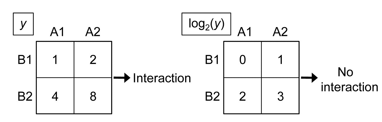
The data matrix for variable y demonstrates that there is significant interaction between particle density and day/night factors, because the means are not additive: the difference in clearance rate between high and low density is not the same during the night (1) as during the day (4). But a simple log$_2$ transform of y gives the table to the right, in which there is now no interaction between the factors: the difference between logged clearance rate at low and high particle density is the same during both day and night (1). Yet, both these tables are identical if viewed non-parametrically, i.e. with the values replaced by their ranks.
This example is scarcely representative of the typical multivariate abundance matrix but it does illustrate that this simple form of interaction is essentially a parametric construction, based on linear models of adding main effects, interactions and error. Though, as previously mentioned, ‘non-parametric interaction’ is not an altogether invalid concept (see Chapter 16), it cannot be straightforwardly defined. The ANOSIM crossed designs are tests for the presence or otherwise of an effect of factor A; this may be a large effect at one level of another factor B, and smaller ones at its other levels, or it may be a more consistent effect of A at all levels of B – these situations are not distinguished, and one way of viewing these $\overline{R}$ statistics is as combinations of ‘main effects’ and ‘interactions’. What they tell you, robustly, is whether factor A has an overall effect, at least somewhere, having removed all contributions that the other crossed factor(s) could possibly be having. They do not do this by subtracting some estimate under a general linear model of the effect of other terms. Their excision of other factors is more surgical than that: they only ever compare the different levels of A under an identical level for all other combinations of factors. Therefore there can be no equivalent, for example, of the way that in linear models main effects can apparently disappear because interactions ‘in different directions’ cancel them out. An $\overline{R}$ statistic is perfectly meaningful in the presence of interactions. Under the null hypothesis, the component R values making up that average are all approximately zero; where there are effects some or all of those R values become positive. If enough of them do so (or one or two of them do so enough), an effect is detected.
¶ It is to be understood that each dot represents a sample of 282 species abundances (going into the page, if you like). Of course, data is not input into PRIMER in this (3-way) format but in the usual species $\times$ (all) samples worksheet, with areas (1-4), years (73-96) and sites (a-h) identified in the associated factors sheet.