9.2 Univariate case
For purely illustrative purposes, Table 9.1 extracts the counts of a single Thyasira species from the Frierfjord macrofauna data {F}, consisting of four replicates at each of six sites.
Table 9.1. Frierfjord macrofauna {F}. Abundance of a single species (Thyasira sp.) in four replicate grabs at each of the six sites (A–E, G).
| Site: | A | B | C | D | E | G |
|---|---|---|---|---|---|---|
| Replicate | ||||||
| 1 | 1 | 7 | 0 | 1 | 62 | 66 |
| 2 | 4 | 0 | 0 | 8 | 102 | 68 |
| 3 | 3 | 3 | 0 | 5 | 93 | 52 |
| 4 | 11 | 2 | 3 | 13 | 69 | 36 |
| Mean | 4.8 | 3.0 | 0.8 | 6.8 | 81.8 | 55.5 |
| Stand. dev. | 4.3 | 2.9 | 1.5 | 5.1 | 18.7 | 14.8 |
Two features are apparent:
-
the replicates are not symmetrically distributed (they tend to be right-skewed);
-
the replication variance tends to increase with increasing mean, as is clear from the mean and standard deviation (s.d.) values given in Table 9.1.
The lack of symmetry (and thus approximate normality) of the replication distribution is probably of less importance than the large difference in variability; ANOVA relies on an assumption of constant variance across the groups. Fortunately, both defects can be overcome by a simple transformation of the raw data; a power transformation (such as a square root), or a logarithmic transformation, have the effect both of reducing right-skewness and stabilising the variance.
Power transformations
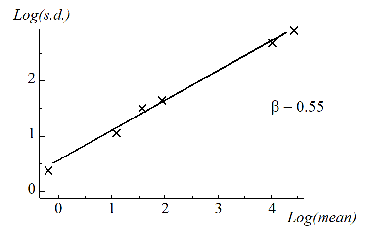
The power transformations $y ^ * = y ^ \lambda$ form a simple and useful family, in which decreasing values of $\lambda$ produce increasingly severe transformations. The log transform, $y ^ * =\log _ e (y)$, can also be encompassed in this series (technically, $(y ^ \lambda-1)/\lambda \rightarrow \log _ e (y)$ as $\lambda \rightarrow 0$). Box & Cox (1964) give a maximum likelihood procedure for optimal selection of $\lambda$ but, in practice, a precise value is not important, and indeed rather artificial if one were to use slightly different values of $\lambda$ for each new analysis. The aim should be to select a transformation of the right order for all data of a particular type, choosing only from, say: none, square root, 4th root or logarithmic. It is not necessary for a valid ANOVA that the variance be precisely stabilised or the non-normality totally removed, just that gross departures from the parametric assumptions (e.g. the order of magnitude change in s.d. in Table 9.1) are avoided. One useful technique is to plot log(s.d.) against log(mean) and estimate the approximate slope of this relationship ($\beta$). This is shown here for the data of Table 9.1.
It can be shown that, approximately, if $\lambda$ is set roughly equal to $1 – \beta$, the transformed data will have constant variance. That is, a slope of zero implies no transformation, 0.5 implies the square root, 0.75 the 4th root and 1 the log transform. Here, the square root is indicated and Table 9.2 gives the mean and standard deviations of the root-transformed abundances: the s.d. is now remarkably constant in spite of the order of magnitude difference in mean values across sites. An ANOVA would now be a valid and effective testing procedure for the hypothesis of ‘no site-to-site differences’, and the means and 95% confidence intervals for each site can be back-transformed to the original measurement scales for a more visually helpful plot.
Table 9.2. Frierfjord macrofauna {F}. Mean and standard deviation over the four replicates at each site, for root-transformed abundances of Thyasira sp.
| Site: | A | B | C | D | E | G |
|---|---|---|---|---|---|---|
| Mean(y*) | 2.01 | 1.45 | 0.43 | 2.42 | 9.00 | 7.40 |
| S.d.(y*) | 0.97 | 1.10 | 0.87 | 1.10 | 1.04 | 1.04 |
Like all illustrations, though genuine enough, this one works out too well to be typical! In practice, there is usually a good deal of scatter in the log s.d. versus log mean plots; more importantly, most species will have many more zero entries than in this example and it is impossible to ‘transform these away’: species abundance data are simply not normally distributed and can only rarely be made so. Another important point to note here is that it is never valid to ‘snoop’ in a data matrix of, perhaps, several hundred species for one or two species that display apparent differences between sites (or times), and then test the significance of these groups for that species. This is the problem of multiple comparisons referred to in Chapter 6; a purely random abundance matrix will contain some species which fallaciously appear to show differences between groups in a standard 5% significance level ANOVA (even were the ANOVA assumptions to be valid). The best that such snooping can do, in hypothesis testing terms, is identify one or two potential key or indicator species that can be tested with an entirely independent set of samples.
These two difficulties between them motivate the only satisfactory approach to most community data sets: a properly multivariate one in which all species are considered in combination in non-parametric methods of display and testing, which make no distributional assumptions at all about the individual counts.

