7.2 Type 2 and type 3 SIMPROF tests
Somerfield & Clarke (2013) describe in full detail a range of useful SIMPROF tests, which they classify as Types 1, 2 and 3. Type 1 SIMPROF has already been seen in Chapter 3 (page 3.5) and is concerned with testing hypotheses, in subsets of the samples, about whether the similarities among those samples show any departure from homogeneity: if all samples appear equally similar to each other, within the bounds of random chance, then there is no basis for further exploration of structure within that subset.
The left-hand side of the schematic below (Fig. 7.2) repeats the steps seen in Chapter 3: the test statistic $\pi$ is the departure of the real similarity profile for that subset (i.e. the ordered set of similarities plotted from smallest to largest) from the average profile expected under the null hypothesis of absence of structure in those samples. Construction of this average (and the variation to be expected about it, under the null) uses permutations of species values over the samples. This Type 1 test is repeated many times for different subsets of samples, e.g. at all nodes of an agglomerative or divisive dendrogram from hierarchical clustering (or even for the groups from the non-hierarchical k-R clustering), seen in Chapter 3 (and 11).
The right-hand side of Fig. 7.2 is concerned with similarities (associations) computed among species, over the full set of samples. Type 2 SIMPROF (top right) tests the hypothesis that no associations of any sort are detectable among all the (retained) species. The test statistic $\pi$ is constructed in exactly the same way, by ordering all the species associations, from smallest to largest to produce a similarity profile, compared against profiles generated under the null hypothesis, by again independently permuting the values for each species across all samples. Clearly such permutations must break down any possible associations of species but, as with all permutation tests, have the immense advantage of retaining exactly the same set of counts (/biomass/cover etc) for each species, so the process is entirely free of any distributional assumptions.
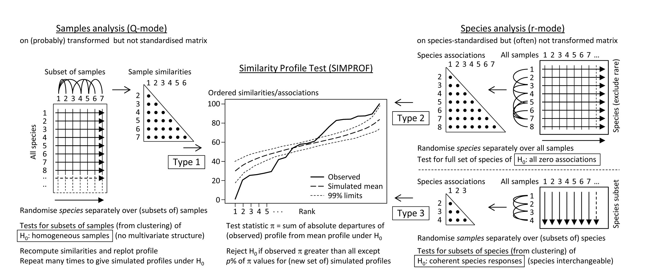
Fig. 7.2. Schematic of the three types of SIMPROF test. Type 1 tests samples (covered earlier) and 2 & 3 test species. Type 2 is a global test of the null hypothesis ($H_0$) of no associations among all species, thus typically carried out only once. Type 3 (as with Type 1) is performed repeatedly in conjunction with some form of cluster analysis (agglomerative, divisive or the non-hierarchical k-R clustering, as in Chapter 3 but applied to the species, not sample similarities) on subdivisions of the species list, to test the null hypothesis of uniformity of species similarities within that sublist. These are best defined by the ‘index of association’. To apply to environmental-type variables (i.e. non-commonly scaled and/or without the need to capture a presence-absence structure, though they may still be biotic), use Pearson or rank correlation for variable similarities. In order for the permutation process to work correctly for Type 3 tests, prior normalisation or ranking is essential (even though these coefficients include a normalisation or ranking step), for the same reason that species standardisation is necessary before employing the index of association (though it includes such standardisation).
Type 2 SIMPROF is therefore designed mainly to be used as a single test, permitting or barring the road to further examination of particular groups of species associations. If the null hypothesis is not rejected, there is no case at all for interpreting a dendrogram such as Fig. 7.1 – we would have no evidence that there were any associations (positive or negative) to interpret. Once we have rejected this specific null for the whole set of species, however, there is no logic in testing it again for a subgroup of those species. What is needed then are tests of a different null hypothesis, that the associations within a subset of species are not distinguishable, i.e. that the species are coherent in their patterns of abundance across the full sample set. In other words, clusters seen in the dendrogram of Fig. 7.1, for example, can be identified statistically as differing in their mutual associations from a wider group of which they are part, but not differentiated internally. This requires a series of Type 3 SIMPROF tests, each as shown in the bottom right of Fig. 7.2, which requires an orthogonal permutation scheme, namely across the subset of species (the species are interchangeable under the null), independently for each sample. Type 3 tests are therefore the natural analogue for species dendrograms of the sequence of Type 1 SIMPROF tests used for sample dendrograms.
Species associations for Exe estuary nematodes
Returning to the Type 2 SIMPROF test, and carrying this out for the Exe estuary nematode data of Fig. 7.1, gives the similarity (association) profile in the main plot of Fig. 7.3, which is seen to differ from profiles under the null both in respect of having many more similarities which are larger (‘positive’ associations) and smaller (‘negative’ associations) than expected. That this is statistically significant, at any probability level we care to nominate, is clear from the histogram of $\pi$ values under the null, in relation to the observed $\pi$ (Fig. 7.3 inset). Note that there are a large number of zero values (fully ‘negative’ associations) in the real profile, but also in all the permuted cases. This is typical of many community matrices: species which occur only in one or two samples are almost certain to be deemed totally dissimilar to other equally sparse species. The difference here is that we have removed many of the sparse species and the real profile is seen to ‘hug the x axis’ longer – it has more species pairs only ever found in different locations than would be expected by chance, as can be seen from Fig. 7.1.
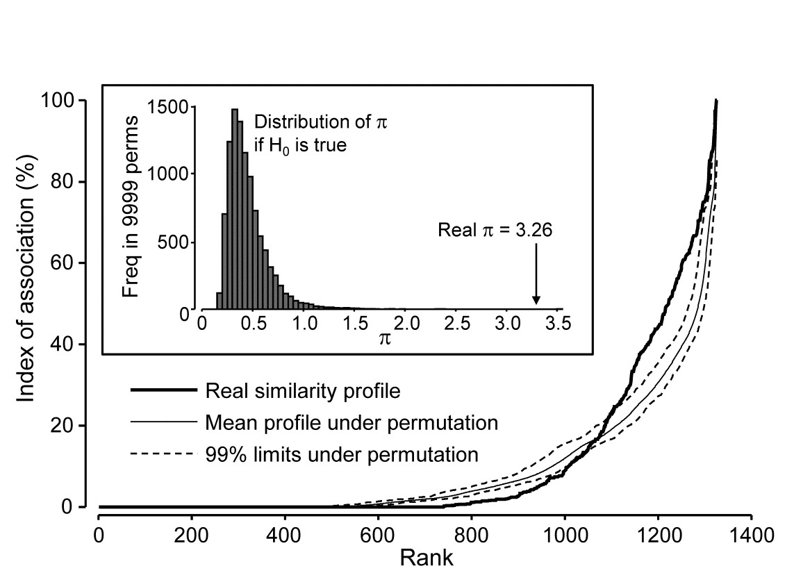
Fig. 7.3. Exe estuary nematodes {X}. Similarity profile (bold line) for a Type 2 SIMPROF test of the null hypothesis of no genuine associations among any of the 52 species making up the dendrogram of Fig. 7.1, consisting of the (52$\times$51)/2 = 1326 indices of association measures computed there, ordered (y axis) and plotted against their ranks (x axis). Also shown, for each value of x, is the mean index (continuous line) from 9999 permutations of the data matrix (under the null hypothesis), and the range (dotted line) in which 99% of the permuted index values lie. Inset: distribution of the distance $\pi$ of (a further) 9999 permuted profiles from the mean profile, in comparison with $\pi$ for the real profile (seen not to come from the null, establishing the existence of species associations).
Type 2 tests can also have a role in testing whether a set of environmental variables may be considered as mutually uncorrelated with each other. The variable ‘similarities’ are then defined as standard Pearson or rank-based Spearman correlations. One might even consider testing a priori designated pairs of variables for evidence of correlation by such a Type 2 permutation method, and this then becomes a distribution-free alternative to Fisher’s z score (or tabulations) for computing significance levels¶. However, systematic testing of large numbers of pairs of variables in this way is probably best avoided: not only is there the problem of repeated testing but also the tests themselves will be highly dependent. This is a familiar theme: the statistics (matrix of correlations) can be extremely useful for interpretation, and the global test (Type 2 SIMPROF) of whether there are any correlations to interpret are key, but the p values for individual correlations must be treated cautiously.
Coherent species curves by Type 3 SIMPROF tests
The procedure is well illustrated by reference to Fig. 7.1, for the reduced set of 52 nematode species from the 19 Exe estuary sites. As we work down from the top of the dendrogram, highly heterogeneous groups (in terms of mixing very low and high associations) gradually give way to sub-groups in which all species are positively associated, though they may not yet be uniformly so, within each subgroup. At one node on each branch the remaining species become totally interchangeable, in the sense that permuting their abundances over that group of species, separately for each sample†, results in more or less the same set of associations: there is no longer significant evidence for any heterogeneity. The non-differentiated species are described as coherent, and no structure is examined below that node. This point may come at quite different similarity levels on each branch – one group might consist of more loosely associated species than another – that is the nature of an exchangeability test. But there is no denying that the results of such a set of Type 3 SIMPROF tests can be profoundly helpful in a key step that has been missing in the exposition so far, namely how to interpret sample patterns in terms of the species that constitute these samples.
To achieve this it is not enough to know how species are grouped; we also need to relate their (common) patterns of abundance to the samples. Here, samples are ordered in keeping with the dendrogram and MDS ordination of samples seen in Chapter 5. The standardised species counts (each species adds to 100 over the 19 sites) are plotted as simple line plots, Fig. 7.4, grouped into the sets identified as internally coherent and externally distinguishable, by the Type 3 tests. These are referred to as coherent species curves, and it is instantly clear that, in this case, the clear clusters seen, for example, in the sample MDS plot (Fig. 5.5) result from a high degree of species turnover among groups of sites, with many of the groups having rather few species in common (or occasionally, none at all).

Fig. 7.4. Exe estuary nematodes {X}. ‘Coherent species curves’, namely groups (A-H) of line plots of relative species abundances, each species standardised (but otherwise untransformed) to total 100% across all 19 sites, and plotted against an arrangement of sites which preserves the sample clustering structure seen in Fig. 5.4. The species groups are identified by a series of SIMPROF (Type 3) tests at the 5% level, on the nodes of the dendrogram of Fig. 7.1, following each branch down from the top until the null hypothesis of coherence (that species below a node are indistinguishable in their associations) cannot be rejected. The later Fig. 7.7 ‘shade plot’ relates these species numbers to respective names, in its redisplay of the dendrogram, with SIMPROF groups identified. Note that groups D and E are plotted together here; they are separated at a higher level of association than found elsewhere and would not have been so by tests with more stringent p values.
Some discussion of the species involved and how the pattern relates to measured environmental differences can be found in Somerfield & Clarke (2013) but, on the methodological front, note that the use of Type 3 SIMPROF tests at a particular significance level is not often a really critical step, as was remarked for the Type 1 tests on page 3.5. E.g. for the data of Fig. 7.4, the same groups are found for tests at the 1% level as at the 5% level. At 0.5%, two group mergers take place: D & E (which are similar and displayed in the same line plot above), and F & G, which fairly reflects the loose grouping of sites 12-19 in the MDS of Fig. 5.5. Pragmatically, the advice is to repeat the tests at three levels and report any minor differences.
¶ For just two variables, the similarity profile reduces to a point but – unlike Type 3 (and Type 1) SIMPROF tests for which all permutations then give a value which is no different than the real one and thus a test is impossible – here the different permutation direction, of the two variables across the full set of samples, gives a full null distribution for this point. In fact the test statistic, $\pi$, is more or less just the absolute value of the correlation coefficient (at least with enough permutations to ensure that the permuted ‘mean profile’ is effectively a point at zero, as it will theoretically be). Another corollary of the permutation direction in Type 2 tests (across samples for each variable) is that there is actually now no need to ‘relativise’ the variables in advance, e.g. by normalising environmental variables or standardising the counts for species, since both correlation and association coefficients include this step internally. However, it is still wise to get into the habit of ‘relativising’ routinely for variable analyses, because it is crucial for Type 3 tests, which otherwise would be meaningless.
† With reference to the previous footnote, it becomes clear at this point exactly why it is necessary to standardise all species across samples before applying the Type 3 SIMPROF permutations: if species have different total abundances then values for a single sample are not meaningfully exchangeable across species, however tightly the patterns of increasing and decreasing abundances over samples may match. The point is obvious for environmental-type variables also, where the permutations might exchange, for example, temperature, salinity and dissolved oxygen values. This could only make sense for normalised variables.