18.3 ‘Bootstrap average’ regions
The idea of the (univariate) bootstrap ( Efron (1979) ) is that our best estimate of the distribution of values taken by the (n) replicates in a single group, if we are not prepared to assume a model form (e.g. normality), is just the set of observed points themselves, each with equal probability (1/n). We can thus construct an example of what a further mean from this distribution would look like – had we been given a second set of n samples from the same group and averaged those – by simply reselecting our original points, independently, one at a time and with equal probability of selection, stopping when we have obtained n values. This is a valid sample from the assumed equi-probable distribution and such reselection with replacement makes it almost certain that several points will have been selected two or more times, and others not at all, and thus the calculated average will differ from that for the original set of n points. This reselection process and recalculation of the mean is repeated as many times (b) as we like, resulting in what we shall refer to as b bootstrap averages. These can be used to construct a bootstrap interval, within which (say) 95% of these bootstrap averages fall. This is not a formal confidence interval as such but gives a good approximation to the precision with which we have determined the average for that group. Under quite general conditions, these bootstrap averages are unbiased for the true mean of the underlying distribution, though their calculated variance underestimates the true variance by a factor of ($1 – n ^ {-1}$); the interval estimate can be adjusted to compensate for this.
Turning to the multivariate case, in the same way we could define ‘whole sample’ bootstrap averages by, in the coral reef context say, reselecting 10 transects with replacement from the 10 replicate transects in one year, and averaging their root-transformed cover values, for each of the 75 species. If this is repeated b = 100 times, separately for each of the years, the resulting 600 bootstrap averages could then be input to Bray-Curtis similarity calculation and metric MDS, which would result in a plot such as Fig. 18.2b. (This is not quite how this figure has been derived but we will avoid a confusing digression at this point, and return to an important altered step on the next page). Fig. 18.2b thus shows the wide range of alternative averages that can be generated in this way. The total possible number of different bootstrap sets of size n from n samples is $(2n)! / [2(n!) ^ 2]$, a familiar formula from ANOSIM permutations and giving again the large number of 92,378 possibilities when there are n = 10 replicates, though the combinations are this time very far from being equally likely.
With such relatively good replication, Fig. 18.2b now gives a clear, intuitively appealing idea both of the relation between the yearly averages and of the limits within which we should interpret the structure of the means. Put simply, all these are possible alternative averages which we could have obtained: if we pick out any two sets of 6, one point from each year in both cases, and would have interpreted the relations among years differently for the two sets, then we are guilty of over-interpreting the data¶. The simplicity of the plot inevitably comes with some caveats, not least that 2-d ordination may not be an accurate representation of the higher-d bootstrap averages. But this is a familiar problem and the solution is as previously: we look at 3-d (or perhaps higher-d) plots. The mMDS in 3-d is shown in Fig. 18.3, and is essentially similar to Fig. 18.2b, though it does a somewhat better job of describing the relative differences between years, as seen by the drop in stress from 0.22 to 0.12 (both are not unduly high for mMDS plots, which will always have much higher stress than the equivalent nMDS – bear in mind that this is an ordination of 600 points!). With balanced replication, as here, one should expect the degree of separation between pairs of bootstrap ‘clouds’ for the different groups to bear a reasonable relationship to the ordering of pairwise ANOSIM R values in Table 18.1, and by spinning the 3-d solution this is exactly what is seen to happen. By comparison, the 2-d plot somewhat under-represents the difference between 1981 and 88 and over-separates 1984 and 87.
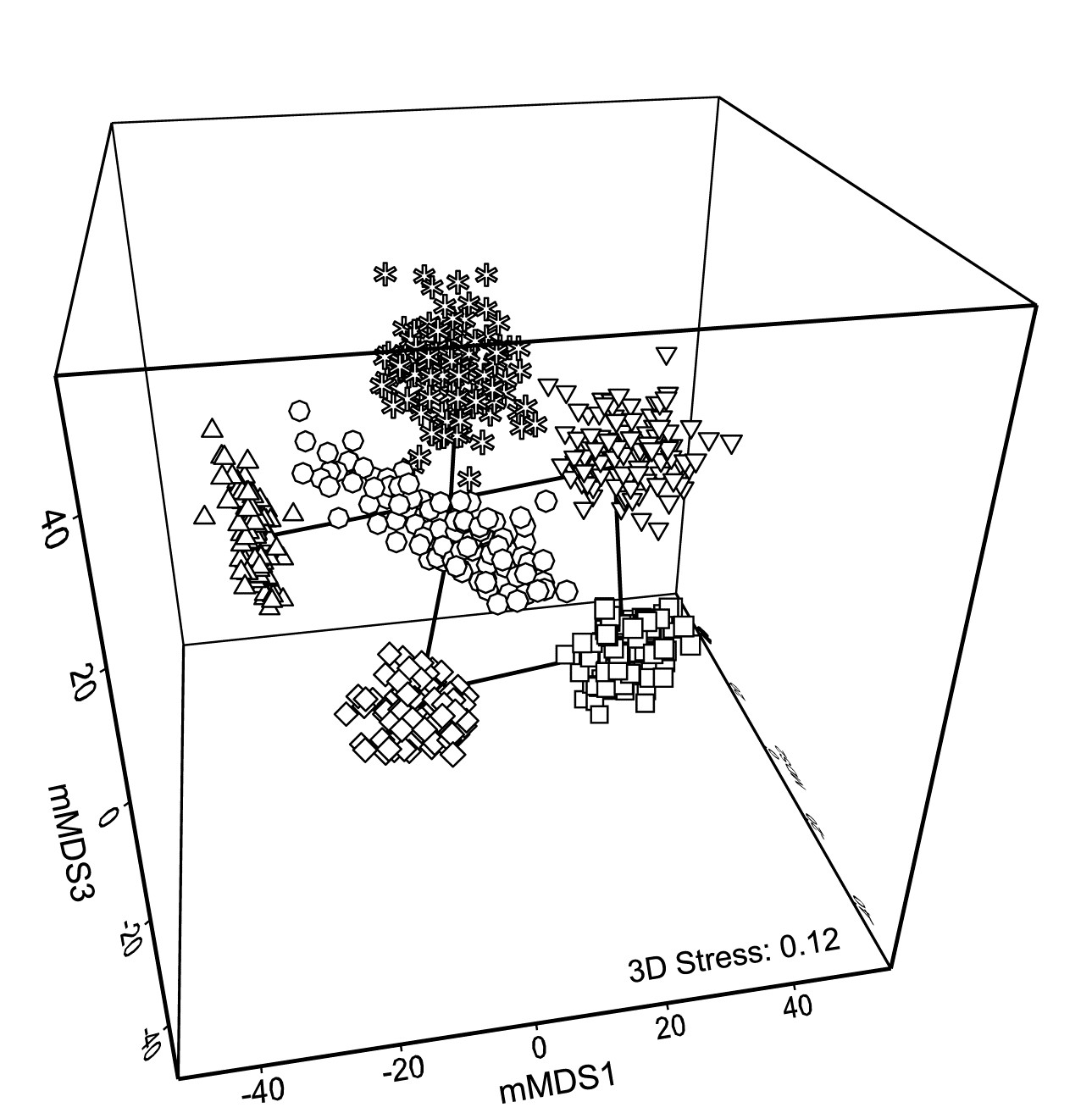
Fig. 18.3. Indonesian reef corals, S. Tikus Island {I} 3-d mMDS of whole sample bootstrap averages constructed as in Fig. 18.2b .
Fig. 18.2c takes the next natural step and constructs smoothed, nominal 95% bootstrap regions on the 2-d plot of Fig. 18.2b. The ordination is unchanged, being still based on the 600 bootstrap averages, the points being suppressed in the display in favour of convex regions describing their spread. These are constructed in a fairly straightforward manner by fitting bivariate normal distributions, with separately estimated mean, variance and correlation parameters to each group of bootstrap averages. Given that each point represents a mean of 10 independent samples, it is to be expected that the ‘cloud’ of bootstrap averages will be much closer to multivariate normality, at least in a space of high enough dimension for adequate representation, than the original single-transect samples. However, non-elliptic contours should be expected in a 2-d ordination space both from any non-normality of the high-dimensional cloud and because of the way the groups interact in this limited MDS display space – some years may be ‘squeezed’ between others. The shifted power transform (of a type used on page 17.9 for the construction of joint $\Delta ^ +$, $\Lambda ^ +$ probability regions) is thus used on a rotation of each 2-d cloud to principal axes, again separately for each group (and axis). The bivariate normals are fitted in the transformed spaces and their 95% contours back transformed to obtain the regions of Fig. 18.2c. Such a procedure cannot generate non-convex regions (as seen for means in 1987, though there is less evidence of non-convexity in the 3-d plot) but often seems to do a good job of summarising the full set of bootstrap averages.
In one important respect the regions are superior to the clouds of points: when the bivariate normals are fitted in the separate transformed spaces, correction can be made for the variance underestimation noted earlier for bootstrap averages in the univariate case. The details are rather involved† but the net effect is to slightly enlarge the regions to cover more than 95% of the bootstrapped averages, to produce the nominal 95% region. The enlargement will be greater as n, the number of replicates for a group, reduces, because the underestimation of variance by bootstrapping is then more substantial.
Fig. 18.2c also allows a clear display of the means for each group. The points (joined by a time trajectory) are the group means of the 100 bootstrap averages in each year, which are merged with those 600 averages, and then ordinated with them into 2-d space. Region plots in the form of Fig. 18.2c thus come closest to an analogue of the univariate means plot, of averages and their interval estimates.
¶ It is likely to be important for such interpretation that we have chosen mMDS rather than nMDS for this ordination. One of the main messages from any such plot is the magnitude of differences between groups compared to the uncertainty in group locations. Metric MDS takes the resemblance scale seriously, relating the distances in ordination space linearly through the origin to the inter-point dissimilarities. As discussed on page 5.8, this is usually a disaster in trying to display complex sample patterns accurately in low-d space because the mMDS ordination has, at the same time, to reconcile those patterns with displaying the full scale of random sampling variability from point to point (samples from exactly the same condition never have 0% dissimilarity). The pattern here is not complex however, just a simple 6 points (with an important indication of the uncertainty associated with each), and the retention of a scale makes mMDS the more useful display.
† An elliptic contour of the bivariate normal is found in the transformed space, with P% cover, where P is greater than the target $P _ 0$ (95%, say), such that the variance bias is countered. A neat simplification results from $P = 100 \left[1 – \left[ 1 – (P _ 0 /100) \right] ^ {1/W} \right]$ for bivariate normal probabilities from concentric ellipses, where W is the bootstrap underestimate of the total variance, from both axes. Under rather general conditions, the expected value of W is again only (1 – n-1), though this cannot be simply substituted into the expression for P since the mean of a function of W is not the function of the mean of W. Hence a large-scale simulation of W is needed to give mean P from the above expression, for a full range of n and a few key $P _ 0$ values. Once computed, the adjustment can be put in a simple look-up table for software (in practice an empirical quadratic fit of P to n-1 suffices), and this is implemented in PRIMER 7’s Bootstrap Averages routine.