15.4 Breakdown of seriation
Clear-cut zonation patterns in the form of a serial change in community structure with increasing water depth are a striking feature of intertidal and shallow-water benthic communities on both hard and soft substrata. The causes of these zonation patterns are varied, and may differ according to circumstances, but include environmental gradients such as light or wave energy, competition and predation. None of these mechanisms, however, will necessarily give rise to discontinuous bands of different assemblages of species, which is implied by the term zonation, and the more general term seriation is perhaps more appropriate for this pattern of community change, zonation (with discontinuities) being a special case.
Many of the factors which determine the pattern of seriation are likely to be modified by disturbances of various kinds. For example, dredging may affect the turbidity and sedimentation regimes and major engineering works may alter the wave climate. Elimination of a particular predator may affect patterns which are due to differential mortality of species caused by that predator. Increased disturbance may also result in the relaxation of interspecific competition, which may in turn result in a breakdown of the pattern of seriation induced by this mechanism. Where a clear sequence of community change along transects is evident in the undisturbed situation, the degree of breakdown of this sequencing could provide an index of subsequent disturbance. Clarke, Warwick & Brown (1993) have described a simple non-parametric index of multivariate seriation, and applied it to a study of dredging impact on intertidal coral reefs at Ko Phuket, Thailand {K}.
In 1986, a deep-water port was constructed on the SE coast of Ko Phuket, involving a 10-month dredging operation. Three transects were established across nearby coral reefs (Fig. 15.5), transect A being closest to the port and subject to the greatest sedimentation, partly through escape of fine clay particles through the southern containing wall. Transect C was some 800 m away, situated on the edge of a channel where tidal currents carry sediment plumes away from the reef, and transect B was expected to receive an intermediate degree of sedimentation. Data from surveys of these three transects, perpendicular to the shore, are presented here for 1983, 86, 87 and 88 (see Chapter 16 for later years). Line-samples of 10m were placed parallel to the shore at 10m intervals along the main transect from the inner reef flat to the outer reef edge, 12 lines along each of transects A and C and 17 along transect B. The same transects were relocated each year and living coral cover of each species recorded.

Fig. 15.5. Ko Phuket corals {K}. Map of study site showing locations of transects, A, B and C.
The basic data were root-transformed and Bray-Curtis similarities calculated between every pair of samples within each year/transect combination (C was not surveyed in 1986); the resulting triangular similarity matrices were then input to non-metric MDS (Fig. 15.6). By joining the points in an MDS, in the order of the samples along the inshore-to-offshore transect, one can visualise the degree of seriation, that is, the extent to which the community changes in a smooth and regular fashion, departing ever further from the community at the start of the transect. A measure of linearity of the resulting sequence could be constructed directly from the location of the points in the MDS. However, this could be misleading when the stress is not zero, so that the pattern of relationships between the samples cannot be perfectly represented in 2 dimensions; this will often be the case, as with some of the component plots in Fig. 15.6¶. Again, a better approach is to work with the fundamental similarity matrix that underlies the MDS plots, of whatever dimension.
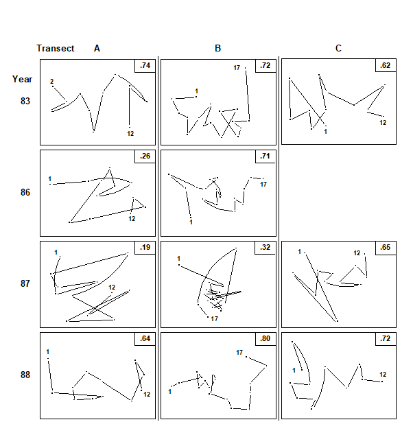
Fig. 15.6. Ko Phuket corals {K}. MDS ordination of the changing coral communities (species cover data) along three transects (A to C) at four times (1983 to 1988). The lines indicate the degree of seriation by linking successive points along a transect, from onshore (1) to offshore samples (12 or 17); $\rho$ values (seriation statistic, IMS) are at top right. Sample 1 from transect A in 1983 is omitted (see text) and no samples were taken for transect C in 1986 (reading across rows, stress = 0.10, 0.11, 0.09; 0.10, 0.11; 0.08, 0.14, 0.11; 0.07, 0.09, 0.10).
The index of multivariate seriation (IMS) proposed is therefore defined as a Spearman correlation coefficient ($\rho _ s$, e.g. Kendall (1970) , see also equation 6.3) computed between the corresponding elements of two triangular matrices of rank ‘dissimilarities’. The first is that of Bray-Curtis coefficients calculated for all pairs from the n coral community samples (n = 12 or 17 in this case). The second is formed from the inter-point distances of n points laid out, equally-spaced, along a line. If the community changes exactly match this linear sequence (for example, sample 1 is close in species composition to sample 2, samples 1 and 3 are less similar; 1 and 4 less similar still, up to 1 and 12 having the greatest dissimilarity) then the IMS has a value $\rho = 1$. If, on the other hand, there is no discernible biotic pattern along the transect, or if the relationship between the community structure and distance offshore is very non-monotonic – with the composition being similar at opposite ends of the transect but very different in the middle – then $\rho$ will be close to zero. These near-zero values can be negative as well as positive but no particular significance attaches to this.
A statistical significance test would clearly be useful, to answer the question: what value of $\rho$ is sufficiently different from zero to reject the null hypothesis of a complete absence of seriation? Such an (exact) test can be derived by permutation in this case. If the null hypothesis is true then the labelling of samples along the transect (1, 2, …, n) is entirely arbitrary, and the spread of $\rho$ values which are consistent with the null hypothesis can be determined by recomputing its value for permutations of the sample labels in one of the two similarity matrices (holding the other fixed). For T randomly selected permutations of the sample labels, if only t of the T simulated $\rho$ values are greater than or equal to the observed $\rho$, the null hypothesis can be rejected at a significance level of 100(t+1)/(T+1)%.†
In 1983, before the dredging operations, MDS configurations (Fig.15.6) indicate that the points along each transect conform rather closely to a linear sequence, and there are no obvious discontinuities in the sequence of community change (i.e. no discrete clusters separated by large gaps); the community change follows a quite gradual pattern. The values of $\rho$ are consequently high (Table 15.5), ranging from 0.62 (transect C) to 0.72 (transect B).
Table 15.5. Ko Phuket corals {K}. Index of Multivariate Seriation ($\rho$) along the three transects, for the four sampling occasions. Figures in parentheses are the % significance levels in a permutation test for absence of seriation (T = 999 simulations).
| Year | Transect A | Transect B | Transect C |
|---|---|---|---|
| 1983 | 0.65 (0.1%) | 0.72 (0.1%) | 0.62 (0.1%) |
| 1986 | 0.26 (3.8%) | 0.71 (0.1%) | – |
| 1987 | 0.19 (6.4%) | 0.32 (0.2%) | 0.65 (0.1%) |
| 1988 | 0.64 (0.1%) | 0.80 (0.1%) | 0.72 (0.1%) |
The correlation with a linear sequence is highly significant in all three cases. Note that in the 1983 MDS for transect A, the furthest inshore sample has been omitted; it had very little coral cover and was an outlier on the plot, resulting in an unhelpfully condensed display of the remaining points. The MDS has therefore been run with this point removed§. There is no similar technical need, however, to remove this sample from the $\rho$ calculation; this was not done in Table 15.5 though doing so would increase the $\rho$ value from 0.65 to 0.74 (as indicated in Fig. 15.6).
On transect A, subjected to the highest sedimentation, visual inspection of the MDS gives a clear impression of the breakdown of the linear sequence for the next two sampling occasions. The IMS is dramatically reduced to 0.26 in 1986, when the dredging operations commenced, although the correlation with a linear sequence is still just significant (p=3.8%). By 1987, $\rho$ on this transect is further reduced to 0.19 and the correlation with a linear sequence is no longer significant. On transect B, further away from the dredging activity, the loss of seriation is not evident until 1987, when the sequencing of points on the MDS configureation breaks down and the IMS is reduced to 0.32, although the latter is still significant (p=0.2%). Note that the MDS plots of Fig. 15.6 may not tell the whole story; the stress values lie between 0.07 and 0.14, indicating that the 2-dimensional pictures are not perfect representations. The largest stress is, in fact, that for transect B in 1987, so that the seriation that is still detectable by the test is only imperfectly seen in the 2-dimensional plot. It is also true that the increased number of points (17) on transect B, in comparison with A and C (12), will lead to a more powerful test. Essentially though what the test is picking up is a tendency for nearby samples on the transect to have more similar assemblages and one should bear in mind in interpreting such analyses that (as with the earlier ANOSIM test) it is the value of the statistic itself which gives the key information here: values around 0.6 or more will only be obtained if there is a clear serial trend in the samples. Smaller, but still significant values could result from serial autocorrelation, which the test will have some limited power to detectȹ.
On transect C there is no evidence of the breakdown of seriation at all, either from the $\rho$ values or from inspection of the MDS plot. By 1988 transects A and B had completely recovered their seriation pattern, with $\rho$ values highly significant (p<0.1%) and of similar size to those in 1983, and clear sequencing evident on the MDS plots. There was clearly a graded response, with a greater breakdown of seriation occurring earlier on the most impacted transect, some breakdown on the middle transect but no breakdown at all on the transect least subject to sedimentation.
Overall, the breakdown in the pattern of seriation was due to the increase in distributional range of species which were previously confined to distinct sections of the shore. This is commensurate with the disruption of almost all the types of mechanism which have been invoked to explain patterns of seriation, and gives us no clue as to which of these is the likely cause.
¶ Even where the stress is low, the well-known arch effect, Seber (1984) , mitigates against a genuinely linear sequence appearing in a 2-d ordination as a straight line; see the footnote on page 11.3. Or to put it a simpler way, given the whole of 2-d space in which to place points which are essentially in sequence (i.e. the distance between points 1 and 2 is less than that between 1 and 3 which is less than between 1 and 4 etc), it is clear that points can ‘snake around’ (without coiling!) in that 2-d space in a large number of possible ways, few of which will end up looking like a straight line. Transect B in Years 83, 86 and 88 are a good case in point: none will be well fitted by a straight line regression on the MDS plot but they clearly have a very strong serial trend.
† The calculations for the tests were carried out using the PRIMER RELATE routine, which is examined in more detail, and in more general form below, when this particular example is concluded. It has been referred to previously in Chapters 6 & 11 ($\rho$ statistic).
§ The problem is discussed on page 5.8 and the solution presented there, mixing a small amount of mMDS stress to the nMDS stress would have been an alternative, effective way of dealing with this.
ȹ The distinction between trend and serial autocorrelation in univariate statistics can be somewhat arbitrary. One can often model a time series just as convincingly by (say) a cubic polynomial response with a simple independent error term as by a simple linear fit with an autocorrelated error structure: which we choose is sometimes a matter of convention. Here, where the non-parametric framework steers clear of any parametric modelling, the test needs to be realistic in ambition: it can demonstrate an effect, and the size of that effect ($\rho$) and the accompanying MDS plot guides interpretation: large values imply a strong serial trend.