2.2 Example: Loch Linnhe macrofauna

A trivial example, used in this and the following chapter to illustrate simple manual computation of similarities and hierarchical clusters, is provided by extracting six species and four years from the Loch Linnhe macrofauna data {L} of Pearson (1975) , seen already in Fig. 1.3 and Table 1.4. (Of course, arbitrary extraction of ‘interesting’ species and years is not a legitimate procedure in a real application; it is done here simply as a means of showing the computational steps.)

Table 2.1. Loch Linnhe macrofauna {L} subset. (a) Abundance (unstransformed) for some selected species and years. (b) The resulting Bray-Curtis similarities between every pair of samples.

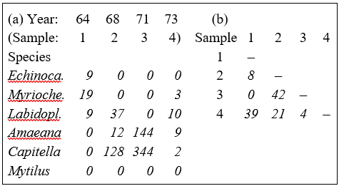
Table 2.1a shows the data matrix of counts and Table 2.1b the resulting lower triangular matrix of Bray-Curtis similarity coefficients. For example, using the first form of equation (2.1), the similarity between samples 1 and 4 (years 1964 and 1973) is:

$$S_{14} = 100 \left[ 1 - \frac{9+16+1+9+2+0}{9+22+19+9+2+0} \right] = 39.3 $$

The second form of equation (2.1) can be seen to give the same result:

$$S_{14} = 100 \left[\frac{2[0+3+9+0+0+0]}{9+22+19+9+2+0} \right] = 39.3 $$

Computation is therefore simple and it is easy to verify that the coefficient possesses the following desirable properties.

a) S = 0 if the two samples have no species in common, since min ($y_{ij}$, $y_{ik}$) = 0 for all i (e.g. samples 1 and 3 of Table 2.1a). Of course, S = 100 if two samples are identical, since |$y_{ij} - y_{ik}$| = 0 for all i.

b) A scale change in the measurements does not change S. For example, biomass could be expressed in g rather than mg or abundance changed from numbers per cm$^2$ of sediment surface to numbers per m$^2$; all y values are simply multiplied by the same constant and this cancels in the numerator and denominator terms of equation (2.1).

c) ‘Joint absences’ also have no effect on S. In Table 2.1a the last species is absent in all samples; omitting this species clearly makes no difference to the two summations in equation (2.1). That similarity should depend on species which are present in one or other (or both) samples, and not on species which are absent from both, is usually a desirable property. As Field, Clarke & Warwick (1982) put it: "taking account of joint absences has the effect of saying that estuarine and abyssal samples are similar because both lack outer-shelf species”. Note that a lack of dependence on joint absences is by no means a property shared by all similarity coefficients.

Transformation of raw data

In one or two ways, the similarities of Table 2.1b are not a good reflection of the overall match between the samples, taking all species into account. To start with, the similarities all appear too low; samples 2 and 3 would seem to deserve a similarity rating higher than 50%. As will be seen later, this is not an important consideration since most of the multivariate methods in this manual depend only on the relative order (ranking) of the similarities in the triangular matrix, rather than their absolute values. More importantly, the similarities of Table 2.1b are unduly dominated by counts for the two most abundant species (4 and 5), as can be seen from studying the form of equation (2.1): terms involving species 4 and 5 will dominate the sums in both numerator and denominator. Yet the larger abundances in the original data matrix will often be extremely variable in replicate samples (the issue of variance structures in community data is returned to in Chapter 9) and it is usually undesirable to base an assessment of similarity of two communities only on the counts for a handful of very abundant species.

The answer is to transform the original y values (the counts, biomass, % cover or whatever) before computing the Bray-Curtis similarities. Two useful transformations are the root transform, $\sqrt{}$y, and the double root (or 4th root) transform, $\sqrt{}\sqrt{}$y. There is more on the effects of transformation later, in Chapter 9; for now it is only necessary to note that the root transform, $\sqrt{}$y, has the effect of down-weighting the importance of the highly abundant species, so that similarities depend not only on their values but also those of less common (‘mid-range’) species. The 4th root transform, $\sqrt{}\sqrt{}$y, takes this process further, with a more severe down-weighting of the abundant species, allowing not only the mid-range but also the rarer species to exert some influence on the calculation of similarity. An alternative severe transformation, with very similar effect to the 4th root, is the log transform, log(1+y).

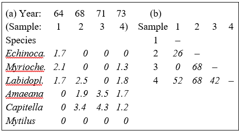
The result of the 4th root transform for the previous example is shown in Table 2.2a, and the Bray-Curtis similarities computed from these transformed abundances, using equation (2.1), are given in Table 2.2b.^‡ There is a general increase in similarity levels but, of more importance, the rank order of similarities is no longer the same as in Table 2.1b (e.g. $S _ {24} > S _ {14}$ and $S _ {34} > S _ {12}$ now), showing that transformations can have a significant effect on the final multivariate display.

Table 2.2. Loch Linnhe macrofauna {L} subset. (a) $\sqrt{}\sqrt{}$-transformed abundance for the four years and six species of Table 2.1. (b) Resulting Bray-Curtis similarity matrix.

In fact, choice of transformation can be more important than level of taxonomic identification (see Chapter 16) especially when abundances are extreme, such as for highly-clumped or schooling species, when dispersion weighting, in place of (or prior to) transformation can be an effective strategy, see Chapter 9.

Canberra coefficient

An alternative which also reduces variability and may sometimes eliminate the need for transformation^§ is to select a similarity measure that automatically balances the weighting given to each species when computed on original counts. One such possibility, the Stephenson, Williams & Cook (1972) form of the so-called Canberra coefficient of Lance & Williams (1967) , defines the similarity between samples j and k as:

$$S_{jk} = 100 \left[ 1 - \frac{1}{p} \sum_{i=1}^{p} \frac{| y_{ij} - y_{ik} | }{( y_{ij} + y_{ik} ) } \right] \tag{2.2}$$

This is another member of the ‘Bray-Curtis family’, bearing a strong likeness to (2.1), but the absolute differences in counts for each species are separately scaled, i.e. the denominator scaling term is inside not outside the summation over species. For example, from Table 2.1a, the Canberra similarity between samples 1 and 4 is:

$$S_{14} = 100 \left[ 1 -\frac{1}{5} \left( \frac{9}{9} + \frac{16}{22} + \frac{1}{19} +\frac{9}{9} +\frac{2}{2} \right) \right] = 24.4 $$

Note that joint absences have no effect here because they are deliberately excluded (since 0/0 is undefined) and p is reset to be the number of species that are present in at least one of the two samples under consideration, an important step for a number of biological measures.

The separate scaling constrains each species to make equal contribution (potentially) to the similarity between two samples. However abundant a species is, its contribution to S can never be more than 100/p, and a rare species with a single individual in each of the two samples contributes the same as a common species with 1000 individuals in each. Whilst there may be circumstances in which this is desirable, more often it leads to overdomination of the pattern by a large number of rare species, of no real significance. (Often the sampling strategy is incapable of adequately quantifying the rarer species, so that they are distributed arbitrarily, to some degree, across the samples.)

Correlation coefficient

A common statistical means of assessing the relationship between two columns of data (samples j and k here) is the standard product moment, or Pearson, correlation coefficient:

$$r_{jk} = \frac{\sum_i ( y_{ij} - \overline{y} _ {\bullet j})( y_{ik} - \overline{y} _ {\bullet k}) } {\sqrt{ \sum_i ( y_{ij} - \overline{y} _ {\bullet j})^2 \sum_i ( y_{ik} - \overline{y} _ {\bullet k})^2}} \tag{2.3}$$

where $ \overline{y} _ {\bullet j}$ is defined as the mean value over all species for the jth sample. In this form it is not a similarity coefficient, since it takes values in the range (–1, 1), not (0, 100), with positive correlation (r near +1) if high counts in one sample match high counts in the other, and negative correlation (r < 0) if high counts match absences. There are a number of ways of converting r to a similarity coefficient, the most obvious for community data being S = 50(1+r).

Whilst correlation is sometimes used as a similarity coefficient, it is not particularly suitable for much biological community data, with its plethora of zero values. For example, it violates the criterion that S should not depend on joint absences; here two columns are more highly positively correlated (and give S nearer 100) if species are added which have zero counts for both samples. If correlation is to be used a measure of similarity, it makes good sense to transform the data initially, exactly as for the Bray-Curtis computation, so that large counts or biomass do not totally dominate the coefficient.

General suitability of Bray-Curtis

The ‘Bray-Curtis family’ is defined by Clarke, Somerfield & Chapman (2006) as any similarity which satisfies all of the following desirable, ecologically-oriented guidelines^¶

a) takes the value 100 when two samples are identical (applies to most coefficients);

b) takes the value 0 when two samples have no species in common (this is a much tougher condition and most coefficients do not obey it);

c) a change of measurement unit does not affect its value (most coefficients obey this one);

d) value is unchanged by inclusion or exclusion of a species which is jointly absent from the two samples (another difficult condition to satisfy, and many coefficients do not obey this one);

e) inclusion (or exclusion) of a third sample, C, in the data array makes no difference to the similarity between samples A and B (several coefficients do not obey this, because they depend on some form of standardisation carried out for each species, by the species total or maximum across all samples);

f) has the flexibility to register differences in total abundance for two samples as a less-than-perfect similarity when the relative abundances for all species are identical (some coefficients standardise automatically by sample totals, so cannot reflect this component of similarity/difference).

In addition, Faith, Minchin & Belbin (1987) use a simulation study to look at the robustness of various similarity coefficients in reconstructing a (non-linear) ecological response gradient. They find that Bray-Curtis and a very closely-related modification (also in the Bray-Curtis family), the Kulczynski coefficient

$$S_{jk} = 100 \frac{\sum _ {i=1} ^ p \min ( y_{ij}, y_{ik}) } {2 / \left[ \left( \sum _ {i=1} ^ p y_{ij} \right) ^ {-1} + \left( \sum _ {i=1} ^ p y_{ij} \right) ^ {-1} \right] } \tag{2.4}$$

Kulczynski (1928) , perform most satisfactorily^†.

Coefficients other than Bray-Curtis, which satisfy all of the above conditions, tend either to have counterbalancing drawbacks, such as the Canberra measure’s forced equal weighting of rare and common species, or to be so closely related to Bray-Curtis as to make little practical difference to most analyses, such as the Kulczynski coefficient, which clearly reverts to Bray-Curtis exactly for standardised samples (when sample totals are all 100).

---

^‡ After a range of Pre-treatment options (including transformation) Bray-Curtis is the default coefficient in the PRIMER Resemblance routine, on data defined as type Abundance (or Biomass), but PRIMER also offers nearly 50 other resemblance measures.

^§ This removes all differences across species in terms of absolute mean abundance but does not address erratic differences within species resulting from schooled or clumped arrivals over the samples. The converse is true of dispersion weighting.

^¶ They are not, of course, universally accepted as desirable! In non-ecological contexts there may be no concept of zero as a ‘special’ number, which must be preserved under transformation because it indicates absence of a species (and ecological work is often concerned as much with the balance of species that are present or absent, as it is with the numbers of individuals found). Even in ecological contexts, some authors prefer not to use a coefficient which has a finite limit (100% = perfect dissimilarity), in part because of technical difficulties this may cause for parametric or semi-parametric modelling when there are many samples with no species in common. These technical issues do not arise for the flexible rank-based methods advocated here (such as non-metric multi-dimensional scaling ordination).

^† This is simply the second form of the Bray-Curtis definition in (2.1), with the denominator terms of the arithmetic mean of the two sample totals across species, $(f+g)/2$, being replaced with a harmonic mean, $2/ ( f^{-1} + g^{-1} )$. In the current authors’ experience, this behaves slightly less well than Bray-Curtis because of the way a harmonic mean is strongly dragged towards the smallest of the totals f and g. Clarke, Somerfield & Chapman (2006) define an intermediate option (also therefore in the Bray-Curtis family) which has a geometric mean divisor $(fg) ^ {0.5}$. This is termed quantitative Ochiai because it reduces to a well-known measure ( Ochiai (1957) ) when the data are only of presences or absences. The serious point here is that it is sufficiently easy to produce new, sensible similarity coefficients that some means of summarising their ‘similarity’ to each other, in terms of their effects on a multivariate analysis, is essential. This is deferred until the 2nd stage plots of Chapter 16.