17.12 Examples
Example: Island fish species lists
Fish species lists extracted from FishBase for a selection of 26 world island groups {i} were slimmed down to leave only species that are ‘endemic’ to the total list, in the sense of being found at only one of these 26 locations. This is an artificial construction, clearly, but it makes the point that the presence/absence matrix which results could never be input to species-level multivariate analysis because all locations then have no species in common, i.e. are 100% dissimilar to each other, and the Bray-Curtis resemblance matrix is uninformative. However, if the taxonomic dissimilarity $\Gamma ^ +$ is calculated for this data, the MDS ordination of Fig. 17.19 is obtained.
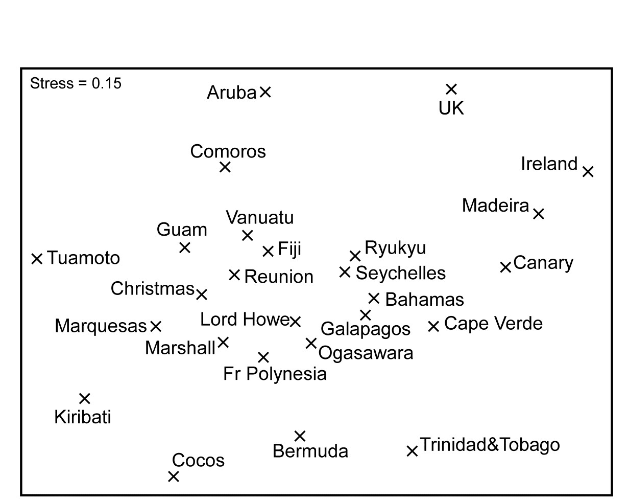
Fig. 17.19. Island group fish species {i}. nMDS ordination from presence/absence data on (pseudo-)endemic species found at 26 island groups, using taxonomic dissimilarity $\Gamma ^ +$.
Whilst this has reasonably high stress, a somewhat interpretable pattern of biogeographic relationships among the island groups is evident.
Example: Valhall oilfield macrofauna
This is another oilfield study, similar to the Ekofisk data ({E}), in which sediment samples are taken at one of five distance groups from the oilfield centre (0.5, 1, 2, 4 and 6 km), in a cross-hair design, and the macrobenthos examined through the time-course of operation of the field (data discussed by Olsgard, Somerfield & Carr (1997) , {V}). The data used here is of 20 samples taken in two years, 1988 and 1991, and the questions of interest concern not just whether a gradient of change exists in the community moving away from the field (which is clear) but whether this gradient is longer – a more accentuated change – in the later year.
After reduction to presence/absence and computation of Bray-Curtis dissimilarity (Sørensen, in effect, see equation 2.7) the nMDS of data from both years in a single ordination is shown in Fig. 17.20a. Whilst it is clear that there is a gradient of change away from the field in a parallel direction for the two years, the most obvious feature is the apparently large change in the community between 1988 and 1991 at all distances, and this certainly makes it difficult to gauge the size of relative changes along the two gradients. This gulf between the two years, e.g. even in the background community at 6km distant from the field, would not be expected at all, and is quite clearly an artefact. It does not take long to realise that the problem was that in 1988 (presumably with less-skilled contractors) the species were not identified with the same degree of discrimination: many species identified only as A in the earlier year had been split into species A and B (or even A, B, C, ..) in the later year, leading to an apparent major increase in species richness! Such an (artefactual) change in the data – an apparent influx of a large number of ‘new’ species – is certain to lead to the wide division of the two years in the MDS. The best solution, of course, is always to work with data at the lowest common denominator of identification: loss of precision in failing to split ‘difficult’ species is usually inconsequential in comparison to artefacts that arise from using inconsistent identification.
Such identification issues can be less obvious than in this case, of course: they may occur infrequently and balance out in terms of numbers of species recorded.

Fig. 17.20. Valhall oilfield macrofauna {V}. nMDS ordinations of macrobenthos from 20 sites in 5 distance groups from the oilfield centre, sampled in 1988 and 1991, using presence/absence data and: a) Bray-Curtis (Sørensen); b) taxonomic dissimilarity $\Gamma ^ +$.
One possibility, if such problems are suspected, is simply to coarsen the data by aggregation to a much higher taxonomic level (Chapter 10), but a less severe course, retaining the finer identification structure, is to use a taxonomic dissimilarity measure. The effect is to say that, whilst species B, C, .. in the later year may not have exact counterparts in the earlier year, they will have a species which is very closely related (species A) and thus contribute little to dissimilarity between the two years. This follows because species which are discriminated to a greater or lesser degree will still usually be placed in the same slightly higher taxonomic group (e.g. genus or family). The dramatic effect of using $\Gamma ^ +$ and not Bray-Curtis on the Valhall data can be seen in Fig. 17.20b. There is still likely to be an artefactual gulf between the years, though they are now much closer together; it can be argued that the distant ‘reference’ samples converge to a greater extent, the remaining difference still being identification issues though one cannot rule out some natural time changes over a wide spatial scale. But what is unarguable is that it is much easier to see the relative scale of gradient change with distance, and note that there is no strong evidence for it having lengthened.