8.7 Multiple diversity indices
A large number of different diversity measures can be computed from a single data set and it is relevant to ask if anything is achieved by doing so. The classic ‘spot’ (alpha) diversity indices, many of which were listed earlier in equations (8.1) to (8.7), are all based either on the set of species proportions {$p _ i$}, the total number of species S, or some mix of these two largely unrelated strands of information, and most are therefore mechanistically inter-correlated as a result, i.e. they will be seen to be correlated whatever the set of data for which they are calculated. Of course, for any particular data set, a richness measure such as simple S and a purely relatedness measure such as Simpson’s $1 - \lambda$ may be observed to correlate across samples, e.g. when a contaminant impact removes a wide range of climax community species, replacing them with a smaller number of opportunists which dominate the total numbers (or area cover), so that both richness and evenness indices decline. But this is a biological correlation not a mechanistic one. In other situations S and $1 - \lambda$ may do something quite different, but H′ (Shannon), J′ (Pielou) and $1 - \lambda$ will always be seen to correlate positively, as a result of their definitions.
We can (and should) examine such issues of whether anything is to be gained in calculating further indices by taking a multivariate approach, in contravention to what many ecologists have done for decades, i.e. test and interpret multiple measures (often mechanistically correlated) separately, as if they were providing independent scrutiny of a specific hypothesis (we are not immune from such strictures ourselves!). Though biological in origin, diversity indices are (statistically speaking) ‘environmental-type’ variables in that their distributions are generally rather well-behaved (as a result of the central limit theorem), needing only mild transformation if at all, and normalisation since they are on different measurement scales. The resulting data matrix of multiple indices across all samples can then be input to PCA (Chapter 4) to reveal the ‘true’ dimensionality, i.e. how many uncorrelated axes of information does this set of indices really contain?
As referred to in Chapter 7 on variables analysis, to examine the relationship of variables to each other, a resemblance matrix can be derived which is initially just the correlations over the samples for every pair of indices; Pearson correlation of (perhaps transformed) measures is appropriate. This may include positive or negative values, for example if Simpson is included as a dominance measure $\lambda$, it will be negatively correlated with evenness indices such as $H ^ \prime$ and $J ^ \prime$. But these indices are still considered closely related so similarity is defined as absolute correlation ($\times 100$). MDS on these similarities displays the relationships.
Garroch Head dump-ground macrofauna
Earlier in the chapter we saw the behaviour of some diversity-based constructions for the 12 sites on the E-W transect across the sewage-sludge dumpsite in the Firth of Clyde (1983 data), e.g. the ‘ABC’ method for contrasting abundance and biomass k-dominance curves, summarised in the W statistic of eqn. (8.11). Calculating also a range of standard diversity indices, none of which needed transformation, the normalised full set of 10 measures when input to PCA¶ is seen to contain only two (or at most three) dimensions of uncorrelated information. The first two PCs account for 95.4% of the variance and the first three for 98.2% (if W is omitted, the first two PCs account for 97.3%).
The MDS plot of the diversity index ‘similarities’ is shown in Fig. 8.16 and tells a simple, and universal, story. To the right are the richness measures (S and Margalef’s d) and to the left the evenness measures (Pielou’s $J ^ \prime$ and Simpson, $1 - \lambda$). On the line between them, mixing evenness and richness, Shannon $H ^ \prime$ and its discrete form, Brillouin H, are seen to be close to evenness indices, though they contain a small element of richness. Fisher’s $\alpha$, essentially the steepness of declines seen in the (log series) distributions of the SAD curves, Fig. 8.4, is seen to be a mixture of both elements. Perhaps the initially surprising observation is that the rarefaction estimates (equation 8.6) – the expected number of species for a given number of individuals, here calculated for ‘rarefying’ to 20 and 45 individuals (the most depauperate sample containing only 46 individuals) – is seen not to estimate richness at all here but to mainly reflect sample evenness. This is not so surprising when the construction is considered in more detail: individuals dropped at random until a small percentage are left (most samples have 100’s or 1000’s of individuals), and so the number of species remaining will be dictated by how dominated the community is by just a few species.
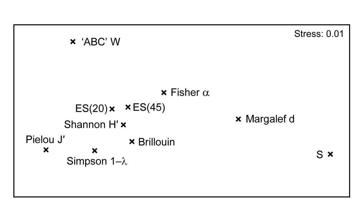
Fig. 8.16. Garroch Head macrofauna {G}. nMDS from absolute Pearson correlations among 10 diversity indices (variables) computed on soft-sediment faunal samples from 12 sites on a transect across the Clyde sewage sludge dump-ground.
Another interesting feature is that the W statistic does not lie on this richness-evenness axis. It is towards the evenness end, as might be expected from its use of the abundance k-dominance curve but here it also provides fresh information from the biomass dominance pattern. And this is the general point that such plots make: whatever the input data matrix, a pattern broadly in line with Fig. 8.16 will emerge. What this plot mainly captures is the mechanistic relationships among the diversity indices rather than the ecological information of a specific context§. The implication is always that the number of diversity indices it makes sense to calculate, based only on the species abundances, is very small – basically one richness and one evenness measure. Striking out from these two axes into third or higher dimensional diversity space needs introduction of fresh information, on biomass patterns perhaps or, for genuinely unrelated dimensions, the concept of average distinctness of a species set, for a given numbers of species, in terms of the taxonomic or genetic/phylogenetic relatedness of the species (or, indeed, their functional relatedness). Such a concept of diversity is returned to in Chapter 17.
¶ More detailed working of PCA for an index set from this data is shown in the PRIMER User Manual, e.g. the extent to which the diversity measures capture the impact gradient seen in the full multivariate analysis, and the definition of the PCs as an overall decline in all diversity measures when sites near the dump centre (PC1) and a contrast between evenness and richness (PC2).
§ A similar idea is seen for ordination of the relationship among competing definitions of distance or dissimilarity, utilising second stage plots (Chapter 16), viz. which coefficients capture the same, and which very different information on multivariate structure?