15.3 Increased variability

Warwick & Clarke (1993b) noted that, in a variety of environmental impact studies, the variability among samples collected from impacted areas was much greater than that from control sites. The suggestion was that this variability in itself may be an identifiable symptom of perturbed situations. The four examples examined were:

1. Meiobenthos from a nutrient-enrichment study {N}; a mesocosm experiment to study the effects of three levels of particulate organic enrichment (control, low dose and high dose) on meiobenthic community structure (nematodes plus copepods), using four replicate box-cores of sediment for each treatment.
    

2. Macrobenthos from the Ekofisk oil field, N Sea {E}; a grab sampling survey at 39 stations around the oil field centre. To compare the variability among samples at different levels of pollution impact, the stations were divided into four groups (A-D) with approximately equal variability with respect to pollution loadings. These groups were selected from a scatter plot of the concentrations of two key pollution-related environmental variables, total PAHs and barium. Since the dose/response curve of organisms to pollutant concentrations is usually logarithmic, the values of these two variables were log-transformed.
    

3. Corals from S Tikus Island, Indonesia {I}; changes in the structure of reef-coral communities between 1981 and 1983, along ten replicate line transects, resulting from the effects of the 1982–83 El Niño.
    

4. Reef-fish in the Maldive Islands {M}; the structure of fish communities on reef flats at 23 coral sites, 11 of which had been subjected to mining, with the remaining 12 unmined sites acting as controls.
    

Data were analysed by non-metric MDS using the Bray-Curtis similarity measure and either square root (mesocosm, Ekofisk, Tikus) or fourth root (Maldives) transformed species abundance data (Fig. 15.4). While the control and low dose treatments in the meiofaunal mesocosm experiment show tight clustering of replicates, the high dose replicates are much more diffusely distributed (Fig. 15.4a). For the Ekofisk macrobenthos, the Group D (most impacted) stations are much more widely spaced than those in Groups A–C (Fig. 15.4b). For the Tikus Island corals, the 1983 replicates are widely scattered around a tight cluster of 1981 replicates (Fig. 15.4c)^¶, and for the Maldives fish the control sites are tightly clustered entirely to the left of a more diffuse cluster of replicates of mined sites (Fig. 15.4d). Thus, the increased variability in multivariate structure with increased disturbance is clearly evident in all examples.
 

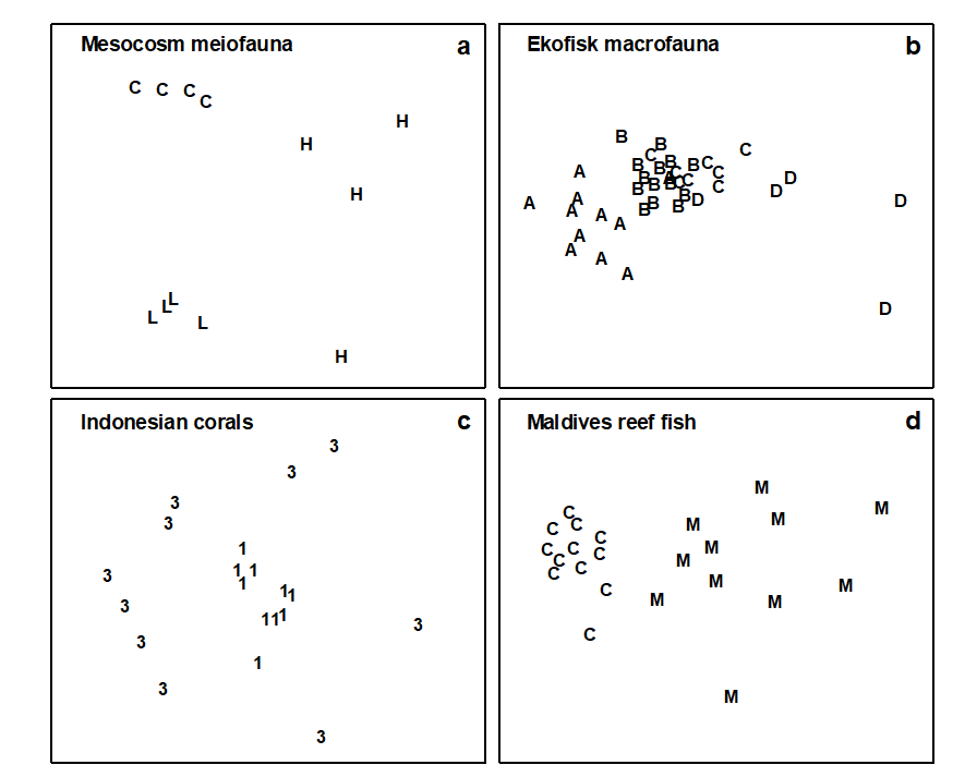
Fig. 15.4. Variability study {N, E, I, M}. Two-dimensional configurations for MDS ordinations of the four data sets. Treatment codes: a) H = High dose, L = Low dose, C = Controls; b) A–D are the station groupings by pollution load; c) 1 = 1981, 3 = 1983; d) M = Mined, C = Controls (stress: 0.08, 0.12, 0.11, 0.08).

It is possible to construct an index from the relative variability between impacted and control samples. One natural comparative measure of dispersion would be based on the difference in average distance among replicate samples for the two groups in the 2-d MDS configuration. However, this configuration is usually not an exact representation of the rank orders of similarities between samples in higher dimensional space. These rank orders are contained in the triangular similarity matrix which underlies any MDS. (The case for using this matrix rather than the distances is the same as that given for the ANOSIM statistic in Chapter 6.) A possible comparative Index of Multivariate Dispersion (IMD) would therefore contrast the average rank of the similarities among impacted samples ($\overline{r} _ t$) with the average rank among control samples ($\overline{r} _ c$) , having re-ranked the full triangular matrix ignoring all between-treatment similarities. Noting that high similarity corresponds to low rank similarity, a suitable statistic, appropriately standardised, is:

$$ IMD = 2 ( \overline{r} _ t - \overline{r} _ c ) / ( N _ t + N _ c) \tag{15.2} $$

where

$$ N _ c = n_ c (n _ c – 1)/2, \hspace{10mm} N _ t = n _ t (n _ t – 1)/2 \tag{15.3} $$

and $n _ c$, $n _ t$ are the number of samples in the control and treatment groups respectively. The chosen denominator ensures that IMD has maximum value of +1 when all similarities among impacted samples are lower than any similarities among control samples. The converse case gives a minimum for IMD of –1, and values near zero imply no difference between treatment groups.

In Table 15.2, IMD values are compared between each pair of treatments or conditions for the four examples. For the mesocosm meiobenthos, comparisons between the high dose and control treatments and the high dose and low dose treatments give the most extreme IMD value of +1, whereas there is little difference between the low dose and controls. For the Ekofisk macrofauna, strongly positive values are found in comparisons between the group D (most impacted) stations and the other three groups. It should be noted however that stations in groups C, B and A are increasingly more widely spaced geographically. Whilst groups B and C have similar variability, the degree of dispersion increases between the two outermost groups B and A, probably due to natural spatial variability. However, the most impacted stations in group D, which fall within a circle of 500 m diameter around the oil-field centre, still show a greater degree of dispersion than the stations in the outer group A which are situated outside a circle of 7 km diameter around the oil-field. Comparison of the impacted versus control conditions for both the Tikus Island corals and the Maldives reef-fish gives strongly positive IMD values. For the Maldives study, the mined sites were more closely spaced geographically than the control sites, so this is another example for which the increased dispersion resulting from the anthropogenic impact is ‘working against’ a potential increase in variability due to wider spacing of sites. Nonetheless, for both the Ekofisk and Maldives studies the increased dispersion associated with the impact more than cancels out that induced by the differing spatial scales.

Table 15.2. Variability study {N, E, I, M}. Index of Multivariate Dispersion (IMD) between all pairs of conditions.

Study	Conditions compared	IMD
Meiobenthos	High dose / Control	+1
	High dose / Low dose	+1
	Low dose / Control	-0.33
Macrobenthos	Group D / Group C	+0.77
	Group D / Group B	+0.80
	Group D / Group A	+0.60
	Group C / Group B	-0.02
	Group C / Group A	-0.50
	Group B / Group A	-0.59
Corals	1983 / 1981	+0.84
Reef-fish	Mined / Control reefs	+0.81

 

Application of the comparative index of multivariate dispersion (the MVDISP routine in PRIMER) suffers from the lack of any statistical framework for testing hypotheses of comparable variability among groups^§. As given above, it is also restricted to the comparison of only two groups, though it can be extended to several groups in straightforward fashion. Let $\overline{r} _ i $ denote the mean of the $N _ i = n _ i ( n _ i – 1)/2$ rank similarities among the $n _ i$ samples within the ith group (i = 1, …, g), having (as before) re-ranked the triangular matrix ignoring all between-group similarities, and let N be the number of similarities involved in this ranking ($N = \sum _ i N _ i$). Then the dispersion sequence

$$ \overline{r} _ 1 /k, \hspace{3mm} \overline{r} _ 2 /k, \ldots \overline{r} _ g /k \tag{15.4} $$

defines the relative variability within each of the g groups, the larger values corresponding to greater within-group dispersion. The denominator scaling factor k is (N + 1)/2, i.e. simply the mean of all N ranks involved, so that a relative dispersion of unity corresponds to ‘average dispersion’. (If the number of samples is the same in all groups then the values in equation (15.4) will average 1, though this will not quite be the case if the {$n _ i$} are unbalanced.)

Table 15.3. Variability study {N, E, I, M}. Relative dispersion of the groups (equation 15.4) in each of the four studies.

Meiobenthos	Control	0.58
	Low dose	0.79
	High dose	1.63
Macrobenthos	Group A	1.34
	Group B	0.79
	Group C	0.81
	Group D	1.69
Corals	1981	0.58
	1983	1.42
Reef-fish	Control reefs	0.64
	Mined reefs	1.44

As an example, the relative dispersion values given by (15.4) have been computed for the four studies (Table 15.3). This is complementary information to the IMD values; Table 15.2 provides the pairwise comparisons which follow the global picture in Table 15.3. The conclusions from the latter are, of course, consistent with the earlier discussion, e.g. the increase in variability at the outermost sites in the Ekofisk study, because of their greater geographical spread, being nonetheless smaller than the increased dispersion at the central, impacted stations.

These four examples all involve either experimental or spatial replication but a similar phenomenon can also be seen with temporal replication. Warwick, Ashman, Brown et al. (2002) report a study of macrobenthos in Tees Bay, UK, for annual samples (taken at the same two times each year) over the period 1973–96 {t}. This straddled a significant, and widely reported, phase shift in planktonic communities in the N Sea, in about 1987. The multivariate dispersion index (IMD), contrasting pre-1987 with post-1987, showed a consistent negative value (increase in inter-annual dispersion in later years) for each of six locations in Tees Bay, at each of the two sampling times (Table 15.4).

Table 15.4. Tees Bay macrobenthos {t}. Index of Multivariate Dispersion (IMD) between pre- and post-1987 years, before/after a reported change in N Sea pelagic assemblages.

	March	September
Area 0	–0.15	–0.15
Area 1	–0.09	–0.60
Area 2	–0.33	–0.33
Area 3	–0.35	–0.36
Area 4	–0.28	–0.67
Area 6	–0.46	–0.15

---

^¶ We shall explore this data set in more detail in Chapter 16, in connection with the effect that choice of different resemblance measures has on the ensuing multivariate analyses. It is crucial to realise that this multivariate dispersion (seen in the MDS plot) represents variability in similarities among different replicate pairs and is not much influenced by, e.g., absolute variation in total cover. Euclidean distance, which is strongly influenced by the latter, shows the opposite pattern, with the replicates widely varying for 1981 and much tighter for 1983. Here, Bray-Curtis is driven by the turnover in species present (a concept ignored by Euclidean distance) in what is a sparse assemblage by 1983.

^§ This is because there is no exact permutation process possible under a null hypothesis which says that dispersion is the same but location of the groups may differ. The only viable route to a test is firstly to estimate the locations of each group in some high-d ‘resemblance space’, and move those group centroids on top of each other. Having removed location differences, permuting the group labels becomes permissible under the null hypothesis. This is the procedure carried out by the PERMDISP routine in PERMANOVA+, Anderson (2006) . Like most tests in this add-on software it is therefore an approximate rather than exact permutation test (because of the estimation step) and is semi-parametric not non-parametric (based on similarities themselves not their ranks).