2.5 Dissimilarity coefficients
The converse concept to similarity is that of dissimilarity, the degree to which two samples are unlike each other. As previously stated, similarities (S) can be turned into dissimilarities ($\delta$), simply by:
$$ \delta = 100 -S \tag{2.11} $$
which of course has limits $\delta = 0$ (no dissimilarity) and $\delta = 100$ (total dissimilarity). $\delta$ is a more natural starting point than S when constructing ordinations, in which dissimilarities between pairs of samples are turned into distances (d) between sample locations on a ‘map’ – the highest dissimilarity implying, naturally, that the samples should be placed furthest apart.
Bray-Curtis dissimilarity is thus defined by (2.1) as:
$$\delta_{jk} = 100 \frac{\sum_{i=1}^{p} | y_{ij} - y_{ik} | }{\sum_{i=1}^{p} ( y_{ij} + y_{ik} ) } \tag{2.12}$$
However, rather than conversion from similarities, other important measures arise in the first place as dissimilarities, or more often distances, the key difference between the latter being that distances are not limited to a finite range but defined over (0, $\infty$). They may be calculated explicitly or have an implicit role as the distance measure underlying a specific ordination method, e.g. as Euclidean distance is for PCA (Principal Components Analysis, Chapter 4) or chi-squared distance for CA (Correspondence Analysis).
Euclidean distance
The natural distance between any two points in space is referred to as Euclidean distance (from classical or Euclidean geometry). In the context of a species abundance matrix, the Euclidean distance between samples j and k is defined algebraically as:
$$d_{jk} = \sqrt{\sum_{i=1}^{p} ( y_{ij} - y_{ik} )^2 } \tag{2.13}$$
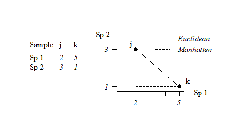
This can best be understood, geometrically, by taking the special case where there are only two species so that samples can be represented by points in 2-dimensional space, namely their position on the two axes of Species 1 and Species 2 counts. This is illustrated below for a simple two samples by two species abundance matrix. The co-ordinate points (2, 3) and (5, 1) on the (Sp. 1, Sp. 2) axes are the two samples j and k. The direct distance $d_{jk}$ between them of $\sqrt{(2–5)^2 + (3–1)^2}$ (from Pythagoras) clearly corresponds to equation (2.13).
It is easy to envisage the extension of this to a matrix with three species; the two points are now simply located on 3-dimensional species axes and their straight line distance apart is a natural geometric concept. Algebraically, it is the root of the sums of squared distances apart along the three axes, equation (2.13) –Pythogoras applies in any number of dimensions! Extension to four and higher numbers of species (dimensions) is harder to envisage geometrically, in our 3-dimensional world, but the concept remains unchanged and the algebra is no more difficult to understand in higher dimensions than three: additional squared distances apart on each new species axis are added to the summation under the square root in equation (2.13). In fact, this concept of representing a species-by-samples matrix as points in high-dimensional species space is a very fundamental and important one and will be met again in Chapter 4, where it is crucial to an understanding of Principal Components Analysis.
Manhattan distance
Euclidean distance is not the only way of defining distance apart of two samples in species space; an alternative is to sum the distances along each species axis:
$$d_{jk} = \sum_{i=1}^{p} | y_{ij} - y_{ik} | \tag{2.14}$$
This is often referred to as Manhattan (or city-block) distance because in two dimensions it corresponds to the distance you would have to travel to get between any two locations in a city whose streets are laid out in a rectangular grid. It is illustrated in the simple figure above by the dashed lines. Manhattan distance is of interest here because of its obvious close affinity to Bray-Curtis dissimilarity, equation (2.12). In fact, when a data matrix has initially been sample standardised (but not transformed), Bray-Curtis dissimilarity is just (half) the Manhattan distance, since the summation in the bottom line of (2.12) then always takes the value 200.
In passing, it is worth noting a point of terminology, though not of any great practical consequence for us. Euclidean and Manhattan measures, equations (2.13) and (2.14), are known as metrics because they obey the triangle inequality, i.e. for any three samples j, k, r:
$$ d _ {jk} + d _ {kr} \ge d_{jr} \tag{2.15} $$
Bray-Curtis dissimilarity does not, in general, satisfy the triangle inequality, so should not be called a metric. However, many other useful coefficients are also not metric distances. For example, the square of Euclidean distance (i.e. equation (2.13) without the $\sqrt{}$ sign) is another natural definition of ‘distance’ which is not a metric, yet the values from this would have the same rank order as those from Euclidean distance and thus give rise, for example, to identical MDS ordinations (Chapter 5). It follows that whether a dissimilarity coefficient is, or is not, a metric is likely to be of no practical significance for the non-parametric (rank-based) strategy that this manual generally advocates.
¶ Though it is of slightly more consequence for the Principal Co-ordinates Analysis ordination, PCO, and the semi-parametric modelling framework of the add-on PERMANOVA+ routines to PRIMER, see Anderson, Gorley & Clarke (2008) , page 110.