8.1 Univariate measures
A variety of different statistics (single numbers) can be used as measures of some attribute of community structure in a sample. These include the total number of individuals (N), total number of species (S), the total biomass (B), and also ratios such as B/N (the average size of an organism in the sample) and N/S (the average number of individuals per species). Abundance or biomass totals (or averages) are not dimensionless quantities so tend to be less informative than diversity indices, such as: richness of the sample, in terms of the number of species (perhaps for a given number of individuals); dominance or evenness in the way in which the total number of individuals in the sample is divided up among the different species (and, in one version of this, a parameter of the species abundance distribution first described by
Fisher, Corbet & Williams (1943)
).
Diversity indices
The main aim is to reduce the multivariate (multi-species) complexity of assemblage data into a single index (or small number of indices) evaluated for each sample, which can then be handled statistically by univariate analyses. It will often be possible to apply standard normal-theory tests (t-tests and ANOVA) to such derived indices (see page 6.1), possibly after transformation.
A bewildering variety of diversity indices has been used, in a large literature on the subject, and some of the most frequently used candidates are listed below.¶ More detail can be found in two (of several) overviews aimed specifically at the biological reader, Heip, Herman & Soetaert (1988) and Magurran (1991) . It should be noted, however, that diversity indices of this type tend to exploit some combination of just two features of the sample information:
a) Species richness. This measure is either simply the total number of species present or some adjusted form which attempts to allow for differing numbers of individuals. Obviously, for samples which are strictly comparable, we would consider a sample containing more species than another to be the more diverse.
b) Equitability. This expresses how evenly the individuals are distributed among the different species, and is often termed evenness. For example, if two samples each comprising 100 individuals and four species had species abundances of 25, 25, 25, 25 and 97, 1, 1, 1, we would intuitively consider the former to be more diverse although the species richness is the same. The former has high evenness, and low dominance (essentially the reverse of evenness), while the latter has low evenness and high dominance (the sample being highly dominated by one species).
Different diversity indices emphasize the species richness or equitability components of diversity to varying degrees. The most commonly used diversity measure is the Shannon (or Shannon–Wiener) diversity index:
$$H^\prime = – \sum _ i p _ i \log(p _ i) \tag{8.1} $$
where $p _ i$ is the proportion of the total count (or biomass etc) arising from the ith species. Note that logarithms to the base 2 are sometimes used in the calculation, reflecting the index’s genesis in information theory. There is, however, no natural biological interpretation here, so the more usual natural logarithm (to the base e) is probably preferable, and commonly used. Clearly, when comparing published indices it is important to check that the same logarithm base has been used in each case. If not, it is simple to convert between results since $\log _ 2 x = (\log _ e x ) / (\log_e 2)$, i.e. all indices just need to be multiplied or divided by a constant factor. Whether it is sensible to compare $H ^ \prime$ across different studies is another matter, since Chapter 17 shows that, like many of the indices given here (Simpson being a notable exception, Fig. 17.1), it can be sensitive to the degree of sampling effort. Hence $H ^ \prime$ should only be compared across equivalent sampling designs.
Species richness
Species richness is often given simply as the total number of species (S), which is obviously very dependent on sample size (the bigger the sample, the more species there are likely to be). Alternatively, Margalef’s index (d) is used, which also incorporates the total number of individuals (N), in an attempt to adjust for the fact that within a larger number of individuals, more species may expect to be found:
$$ d = (S-1) / \log N \tag{8.2} $$
Equitability
This is often expressed as Pielou’s evenness index:
$$ J^ \prime = H ^ \prime / H ^ \prime _ {max} = H ^ \prime / \log S \tag{8.3} $$
where $H ^ \prime _ {max}$ is the maximum possible value of Shannon diversity, i.e. that which would be achieved if all species were equally abundant (namely, log S).
Simpson
Another commonly used measure is the Simpson index, which has a number of forms:
$$ \lambda = \sum p _ i ^ 2 $$ $$ 1 - \lambda = 1 - \left( \sum p _ i ^ 2 \right) $$ $$ \lambda ^ \prime = \left( \sum _ i N _i (N _ i -1) \right) / \left[ N ( N -1) \right] $$ $$ 1 - \lambda ^ \prime = 1 - \left( \sum _ i N _i (N _ i -1) \right) / \left[ N ( N -1) \right] \tag{8.4} $$
where $N _ i$ is the number of individuals of species i. The index $\lambda$ has a natural interpretation as the probability that any two individuals from the sample, chosen at random, are from the same species ($\lambda$ is always $ \le 1$). It is a dominance index, in the sense that its largest values correspond to assemblages whose total abundance is dominated by one, or a very few, of the species present. Its complement, $1 – \lambda$, is thus an equitability or evenness index (sometimes called Gini-Simpson), taking its largest value (of $1 – S ^ {–1}$) when all species have the same abundance. The slightly revised forms $\lambda ^ \prime$ and $1 – \lambda ^ \prime$ are appropriate when total sample size (N) is small (they correspond to choosing the two individuals at random without replacement rather than with replacement). As with Shannon, Simpson diversity can be employed when the {$p_i$} come from proportions of biomass, standardised abundance or other data that are not strictly integral counts but, in that case, the $\lambda ^ \prime$ and $1 – \lambda ^ \prime$ forms are not appropriate.
Other count-based measures
Further well-established indices include that of Brillouin (see Pielou (1975) ):
$$H = N ^ {–1} \log _ e \left( N!/[N _ 1! N _ 2! \ldots N _ S!] \right) \tag{8.5} $$
and a further model-based description, Fisher’s $\alpha$ ( Fisher, Corbet & Williams (1943) ), which is the shape parameter, fitted by maximum likelihood, under the assumption that the species abundance distribution (SAD curve) follows a log series distribution. This has certainly been shown to be the case for some ecological data sets but can by no means be universally assumed, and (as with Brillouin) its use is clearly restricted to genuine (integral) counts.
The final option in this category is the rarefaction method of Sanders (1968) and Hurlbert (1971) , which under the strict assumption that individuals arrive in the sample independently of each other, can be used to project back from the counts of total species (S) and individuals (N), how many species ($E S _ n$) would have been ‘expected’ had we observed a smaller number (n) of individuals:
$$ E S _ n = \sum _ {i=1} ^ S \left[ 1 - \frac{ ( N - N _ i ) ! ( N - n ) ! }{ ( N - N _ i -n) ! N !} \right] \tag{8.6} $$
The idea is thereby to generate an absolute measure of species richness, say $E S _ {100}$ (the number of different species ‘expected’ in a sample of 100 individuals), which can be compared across samples of very differing sizes. It must be admitted, however, that the independence assumption is practically unrealistic. It corresponds to individuals from each species being spatially randomly distributed, giving rise to independent Poisson counts in replicate samples. This is rarely observed in practice, with most species exhibiting some form of spatial clustering, which can often be extreme. Rarefaction will then be strongly biased, consistently overestimating the expected number of species for smaller sample sizes.
Hill numbers
Finally, Hill (1973b) proposed a unification of several diversity measures in a single statistic, which includes as special cases:
$$ N _ 0 = S $$ $$ N _ 1 = \exp( H ^ \prime) $$ $$ N _ 2 = 1 / \sum p _ i ^ 2 $$ $$ N _ \infty = 1 / \max (p _ i ) \tag{8.7} $$
$N _ 1$ is thus a transform of Shannon diversity, $N _ 2$ the reciprocal of Simpson’s dominance $\lambda$ (called inverse Simpson) and $ N _ \infty$ is another possible evenness index (the reciprocal of the Berger-Parker index), which takes larger values if no single species dominates the total abundance. Other variations on these Hill numbers are given by
Heip, Herman & Soetaert (1988)
.
Units of measurement
The numbers of individuals belonging to each species are the most common units used in the calculation of the above indices. For internal comparative purposes other units can sometimes be used, e.g. biomass or total cover of each species along a transect or in quadrats (e.g. for hard-bottom epifauna), but obviously diversity measures using different units are not difficult to compare. Often, on hard bottoms where colonial encrusting organisms are difficult to enumerate, total or percentage cover will be much more realistic to determine than species abundances.
Representing communities
Changes in univariate indices between sites or over time are usually presented graphically† simply as plots of means and confidence intervals for each site or time. For example, Fig. 8.1 graphs the differences in diversity of the macrobenthos and meiobenthic nematodes at six stations in Hamilton Harbour, Bermuda, showing that there are clear differences in diversity between sites for the former but much less obvious differences for the latter. Fig. 8.2 graphs the temporal changes in three univariate indices for reef corals at South Tikus Island, Indonesia, spanning the period of the 1982–3 El Niño (an abnormally long period of high water temperatures which caused extensive coral bleaching in many areas throughout the Pacific). Note the dramatic decline between 1981 and 1983 and subsequent partial recovery in both the number of species ($S$) and the Shannon diversity ($ H ^ \prime$), but no obvious changes in evenness ($ J ^ \prime$).
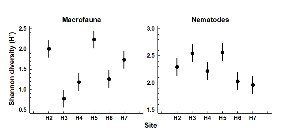
Fig. 8.1. Hamilton Harbour, Bermuda {H}. Diversity (H′) and 95% confidence intervals for macrobenthos (left) and meiobenthic nematodes (right) at six stations.
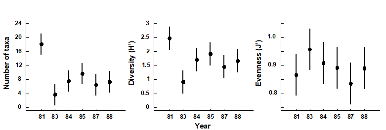
Fig. 8.2. Indonesian reef corals, South Tikus Island {I}. Total number of species (S), Diversity (H') and Evenness (J') based on coral species cover data along transects, spanning the 1982–3 El Niño.
Discriminating sites or times
The significance of differences in univariate indices between sampling sites or times can simply be tested by one-way analysis of variance (ANOVA)§ followed by t-tests or multiple comparison tests for individual pairs of sites; see discussion at the start of Chapter 6.
Determining stress levels
Increasing levels of environmental stress have historically been considered to decrease diversity (e.g. $H ^ \prime$), decrease species richness (e.g. d) and decrease evenness (e.g. $J ^ \prime$), i.e. increase dominance. This interpretation may, however, be an over-simplification of the situation. Subsequent theories on the influence of disturbance or stress on diversity have suggested that in situations where disturbance is minimal, species diversity is reduced because of competitive exclusion between species; with a slightly increased level or frequency of disturbance competition is relaxed, resulting in an increased diversity, and then at still higher or more frequent levels of disturbance species start to become eliminated by stress, so that diversity falls again. Thus it is at intermediate levels of disturbance that diversity is highest (
Connell (1978)
;
Huston (1979)
). Therefore, depending on the starting point of the community in relation to existing stress levels, increasing levels of stress (e.g. induced by pollution) may either result in an increase or decrease in diversity. It is difficult, if not impossible, to say at what point on this continuum the community under investigation exists, or what value of diversity one might expect at that site if the community were not subjected to any anthropogenic stress. Thus, changes in diversity can only be assessed by comparisons between stations along a spatial contamination gradient (e.g. Fig. 8.1) or with historical data (Fig. 8.2).
Caswell’s neutral model
In some circumstances, the equitability component of diversity can, however, be compared with a theoretical expectation for diversity, given the number of individuals and species present. Observed diversity has been compared with predictions from Caswell’s neutral model ( Caswell (1976) ). This model constructs an ecologically ‘neutral’ community with the same number of species and individuals as the observed community, assuming certain community assembly rules (random births/deaths and random immigrations/emigrations) and no interactions between species. The deviation statistic V is then determined which compares the observed diversity ($H ^ \prime$) with that predicted from the neutral model ($E(H ^ \prime)$):
$$ V = \frac{ \left[ H ^ \prime - E (H ^ \prime) \right] }{SD ( H ^ \prime) } \tag{8.8} $$
A value of zero for the V statistic indicates neutrality, positive values indicate greater diversity than predicted and negative values lower diversity. Values > +2 or < -2 indicate ‘significant’ departures from neutrality. The computer program of Goldman and Lambshead (1989) is useful.‡
Table 8.1 gives the V statistics for the macrobenthos and nematode component of the meiobenthos from Hamilton Harbour, Bermuda (c.f. Fig. 8.1). Note that the diversity of the macrobenthos at stations H4 and H3 is significantly below neutral model predictions, but the nematodes are close to neutrality at all stations. This might indicate that the macrobenthic communities are under some kind of stress at these two stations. However, it must be borne in mind that deviation in H′ from the neutral model prediction depends only on differences in equitability, since the species richness is fixed, and that the equitability component of diversity may behave differently from the species richness component in response to stress (see, for example, Fig. 8.2). Also, it is quite possible that the ‘intermediate disturbance hypothesis’ will have a bearing on the behaviour of V in response to disturbance, and increased disturbance may either cause it to decrease or increase. Using this method, Caswell found that the flora of tropical rain forests had a diversity below neutral model predictions!
Table 8.1. Hamilton Harbour, Bermuda {H}. V statistics for summed replicates of macrobenthos and meiobenthic nematode samples at six stations.
| Station | Macrobenthos | Nematodes |
|---|---|---|
| H2 | +0.5 | –0.1 |
| H3 | –5.4 | +0.4 |
| H4 | –4.5 | –0.5 |
| H5 | –1.9 | 0.0 |
| H6 | –1.3 | –0.4 |
| H7 | –0.2 | –0.4 |
¶ The PRIMER DIVERSE routine permits selection of a subset from a list of over 20 indices, sending the values to a worksheet for plotting or export to a mainstream statistical package. Whilst the (non-parametric multivariate) PRIMER package does not do conventional univariate statistical testing, under the usual normality and constant variance assumptions across groups (which can be found in all standard statistical software), some of the elements of univariate analysis are certainly possible, univariate being a special case of multivariate! – see later. PRIMER also has plotting routines for Means Plots, Histograms, Box Plots, Line Plots, Scatter Plots for pairs or triples of indices etc.
† PRIMER 7’s Means Plot produces plots such as Fig. 8.1, the 95% confidence intervals either based on separate estimates of variance for each group or, as throughout this manual, assuming a pooled variance estimate (constant variance) across groups.
§ A rank-based alternative, using PRIMER, would be to compute Euclidean distance on a single variable (index) and input this to ANOSIM. This does not give the usual non-parametric univariate tests (Wilcoxon Mann-Whitney U for two groups, Kruskal-Wallis for several groups), but gives an alternative which generalises to multivariate data in a way that those tests do not, the permutation structure being the same but the test statistics differing. Or using PERMANOVA on the Euclidean distances gives an exact copy of the classical ANOVA table (see Anderson, Gorley & Clarke (2008) ), except that the ‘F tests’ are permutation-based rather than making the less robust F distribution assumption, from normality (but the two will be very similar here, since normality is realistic for most indices).
‡ This is implemented in the PRIMER CASWELL routine, but the significance aspects should be treated with some caution since they are inevitably crucially dependent on the neutral model assumptions. These are usually over-simplistic for real assemblages (even when genuinely neutral, in the sense that their species do not interact) because they again assume simple spatial randomness.