18.5 Example: Fal estuary macrofauna
The soft-sediment macrobenthic communities from five creeks of the Fal estuary, SW England, {f} were examined by Somerfield, Gee & Warwick (1994a) and Somerfield, Gee & Warwick (1994b) . For location of the creeks (Restronguet, Mylor, Pill, St Just, Percuil) see the map in Fig. 9.3, where the analysis was of the sediment meiofaunal assemblages. The sediments in this estuary are heavily contaminated by heavy metal levels, resulting from historic tin and copper mining in the surrounding area, and the macrofaunal species list for the 5 replicates per creek (7 in Restronguet) consists of only 23 taxa. A 2-d metric MDS of these 27 samples, based on fourth-root transformed counts and Bray-Curtis similarity, is seen in Fig. 18.6a, and the associated Shepard plot in 18.6b. In this case, an excellent approximation to the Bray-Curtis resemblances is obtained from the Euclidean distances in an m = 4-dimensional mMDS, for which the Pearson correlation to the Bray-Curtis dissimilarities is $\rho = 0.991$, as seen from the Shepard diagram, Fig. 18.6c.
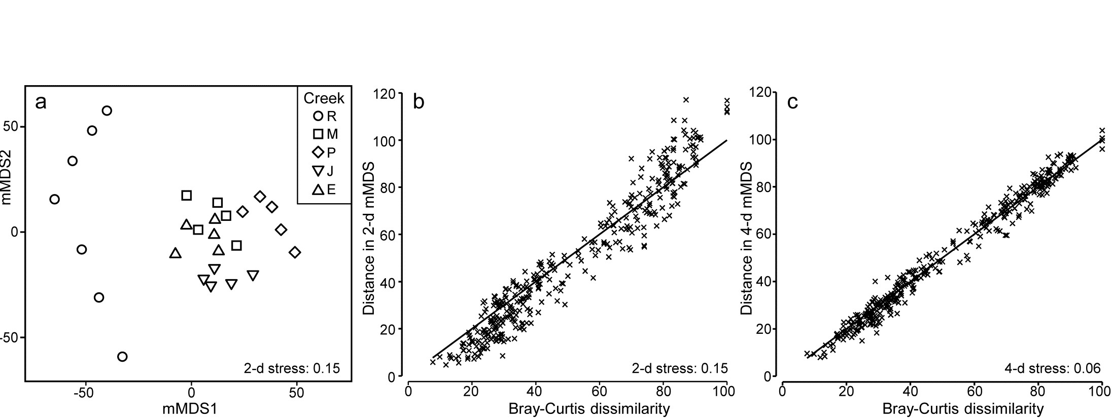
Fig. 18.6. Fal estuary macrofauna {f}. a) mMDS from Bray-Curtis similarities on fourth-root transformed counts of 23 soft-sediment macrofaunal species in a total of 27 samples from 5 creeks of the Fal estuary (R = Restronguet, M = Mylor, P = Pill, J = St Just, E = Percuil); b) Shepard plot for this 2-d mMDS ; c) Shepard plot for a 4-d mMDS of the same data (Pearson correlation = 0.991)
A total of 100 bootstrap averages are generated in this 4-d space, for each creek, and the full set of 500 bootstraps is ordinated into 2-d in Fig. 18.7. Approximate 95% regions are superimposed, in the way outlined earlier. In all cases, fewer than 5 of the 100 bootstrap averages fall outside of these regions, because of the adjustment made to the coverage probability from simulations based on a theoretical bias of ($1 - n ^ {-1}$) in their variance. These adjustments are rather modest however, and cannot be expected to compensate for all sources of potential uncertainty in bootstrapping with small n, and of course displaying in low-d space.
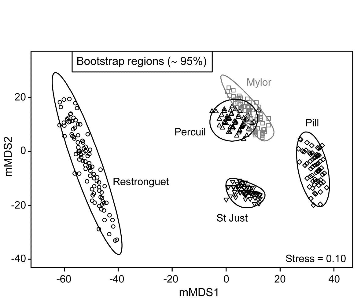
Fig. 18.7. Fal estuary macrofauna {f}. Metric MDS of bootstrap averages for the five creeks from the replicate samples of Fig 8.6a (Mylor creek in grey to aid distinction), including ~95% region estimates for the ‘mean communities’ in each creek. Bootstrapping performed in m = 4 dimensional mMDS space.
It should not be forgotten that the bootstrap concept in univariate space was introduced and justified on the basis of its asymptotic (large n) behaviour. It has some desirable small-sample properties, such as the unbiasedness of bootstrap means for the underlying true mean. But there is no guarantee that, for small n, intervals produced from the percentiles of the set of averages of randomly drawn bootstrap samples will achieve their nominal ‘% cover’. Some authors have even suggested the need for n>50 replicates (for each group!). Whilst this is unrealistic, and unnecessary, it should caution us not to take a nominal 95% cover value too seriously.
One formula worth bearing in mind is that given on page 18.3 for the number of possible different bootstrap averages (B) that could be obtained from n samples, $B = (2n) ! / [2 ( n ! ) ^ 2]$. For n = 2, B = 3; for n=3, B = 10; for n = 4, B = 35; and only when n = 5 do we have more than 100 possibilities (B = 126). At that level, though not all these distinct combinations will be found in b=100 random draws¶, the majority will appear, giving at least a range of bootstrap averages to generate the regions, as can be seen from the Mylor, Pill, St Just and Percuil creeks in Fig. 18.7. (Restronguet, with n=7, has more combinations, B = 1716, and that can be seen in the more random cover of points, rather than the striated patterns of the other bootstraps). Certainly n=5 should be considered as absolutely minimal for such bootstrap regions.
These caveats aside, and minimal though replication may be in the case of Fig. 18.7, it is clear nonetheless that the only two creeks whose regions overlap – and strongly so – are Mylor and Percuil. And pairwise ANOSIM test results, using the original Bray-Curtis similarities, are again consistent with these bootstrap averages: R = -0.01 for the Mylor v. Percuil test, but all other R statistics are > 0.55 and significant at the 1% level. (This level is the most extreme of the 126 permutations possible for all pairwise comparisons of 5 replicates; comparisons with Restronguet, with its 7 replicates, are based on 792 permutations, but all those pairwise tests again return p<1%). Whilst the warning given in the footnote on page 18.4 (that it would be most unwise to use these regions as substitutes for hypothesis tests) is still very germane, it is reassuring to note how often the interpretations broadly concur.
Finally, comparison of Figs. 18.6a and 18.7 restates the point made by the initial Fig. 18.1. In univariate statistics, we do not expect a plot of the replicates themselves to be the most informative way to picture the patterns in a data set. The means plot, with its interval estimates (which are not of course trying to summarise variation in the replicates, but uncertainty in the knowledge of the averages for each group), can often be a more informative way of interpreting the results of hypothesis tests. The same reasoning is true in the multivariate case. Fig. 18.6a has few samples to clutter the basic ordination plot, by comparison with many studies, but the patterns demonstrated by the ANOSIM (or PERMANOVA) tests are then more clearly visualised in a means plot such as Fig. 18.7. To repeat the mantra: test using the replicates, display using the means (with or without bootstrap regions).
¶ They are not equally likely but have a multinomial distribution, thus the probability that a single bootstrap sample will consist of all 5 of one of the original samples is small, at only 1/625, so is unlikely to be seen in most runs of b=100 averages. In contrast, the probability that a bootstrap sample reselects all 5 replicates in the original sample is 24/625 = 0.038, so its average point will occur about 4 times in a run of b=100, and has about a 98% chance of being in the set at least once.