16.2 Matching of ordinations
The BEST (Bio-Env) technique of Chapter 11 can be generalised in a natural way, to the selection of species rather than abiotic variables. The procedure is shown schematically in Fig. 16.2. Here the two starting data sets are not: 1) biotic, and 2) abiotic descriptions of the same set of samples, but: 1) the faunal matrix, and 2) a copy of that same faunal matrix. Variable sets (species) are selected from the second matrix such that their sample ordination matches, ‘as near as makes no difference’, the ordination of samples from the first matrix, the full species set. This matching process, as seen in Chapter 11, best takes place by optimising the correlation between the elements of the underlying similarity matrices, rather than matching the respective ordinations, because of the approximation inherent in viewing inter-sample relationships in only 2-dimensions, say. The appropriate correlation coefficient could be Spearman or Kendall, or some weighted form of Spearman, but there is little to be gained in this context from using anything other than the simplest form, the standard Spearman coefficient ($\rho$).
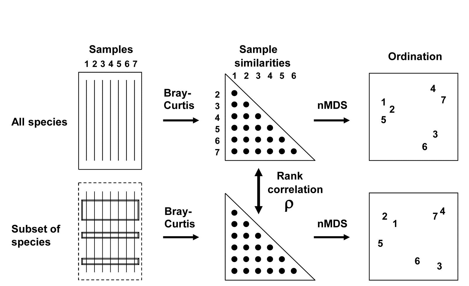
Fig. 16.2. Schematic diagram of selection of a subset of species whose multivariate sample pattern matches that for the full set of species (BEST routine). The search is either over all subsets of the species (Bio-Env option) or, more practically, a stepwise selection of species (BVStep option), aiming to find the smallest subset of species giving rank correlation between the similarity matrices of $\rho \ge 0.95$.
A definition of a ‘near-perfect’ match is needed, and this is (somewhat arbitrarily) deemed to be when $\rho$ exceeds 0.95. Certainly two ordinations from similarity matrices that are correlated at this level will be virtually indistinguishable and could not lead to different interpretation of the patterns. The requirement is therefore to find the smallest possible species subset whose Bray-Curtis similarity matrix correlates at least at $\rho = 0.95$ with the (fixed) similarity matrix for the full set of species.
There is a major snag, however, to carrying over the Bio-Env approach to this context. A search through all possible subsets of 125 species involves: 125 possibilities for a single species, $ _ {125} C _ 2 ( = 125 \times 124 / 2 ) $ pairs of species, $_{125}C _ 3 ( = 125 \times 124 \times 123 / 6) $ triples, etc., and this number clearly gets rapidly out of control. In fact a full search would need to look at $2 ^ {125} – 1$ possible combinations, an exceedingly large number!
Stepwise procedure
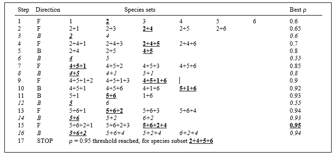
One way round the problem is to search not over every possible combination but some more limited space, and the natural choice here is a stepwise algorithm which operates sequentially and involves both forward and backward-stepping phases.¶ At each stage, a selection is made of the best single species to add to or drop from the existing selected set. Typically, the procedure will start with a null set, picking the best single variable (maximising $\rho$), then adding a second variable which gives the best combination with the first, then adding a third to the existing pair. The backward elimination phase then intervenes, to check whether the first selected variable can now be dropped, the combination of second and third selections alone not having been considered before. The forward selection phase returns and the algorithm proceeds in this fashion until no further improvement is possible by the addition of a single variable to the existing set or, more likely here, the stopping criterion is met ($\rho$ exceeds 0.95). In order fully to clarify the alternation of forward and backward stepping phases, Table 16.1 describes a purely hypothetical (and unrealistically convoluted) search over 6 variables. Analogously to the MDS algorithm of Chapter 6, it is quite possible that such an iterative search procedure will get trapped in a local optimum and miss the true best solution; only a minute fraction of the vast search space is ever examined. Thus, it may be helpful to begin the search at several, different, random starting points, i.e. to start sequential addition or deletion from an existing, randomly selected set of half a dozen (say) of the species.†
Table 16.1. Hypothetical illustration of stages in a stepwise algorithm (F: forward selection, B: backward elimination steps) to select a subset of species which match the multivariate sample pattern for a full set (here, 6 species). Bold underlined type indicates the subset with the highest $\rho$ at each stage, and italics denote a backward elimination step that decreases $\rho$ and is therefore ignored. The procedure ends when $\rho$ attains a certain threshold ($\rho \ge 0.95$), or when forward selection does not increase $\rho$.
¶ This concept may be familiar from stepwise multiple regression in univariate statistics, which tackles a similar problem of selecting a subset of explanatory variables which account for as much as possible of the variance in a single response variable.
† The PRIMER BEST routine (BVStep option) carries out this stepwise approach on an active sheet which is the similarity matrix from all species (Bray-Curtis here), supplying a secondary sheet which is the (transformed) data matrix itself. There are options always to exclude, or always to include, certain variables (species) in the selection, to start the algorithm either with none, all or a random set of species in the initial selection, and to output results of the iteration at various levels of detail (full detail recommended).