11.4 Linking biota to multivariate environmental patterns
The intuitive premise adopted here is that if the suite of environmental variables responsible for structuring the community were known¶, then samples having rather similar values for these variables would be expected to have rather similar species composition, and an ordination based on this abiotic information would group sites in the same way as for the biotic plot. If key environmental variables are omitted, the match between the two plots will deteriorate. By the same token, the match will also worsen if abiotic data which are irrelevant to the community structure are included.†
The Exe estuary nematode data {X} again provides an appropriate example. Fig. 11.7a repeats the species MDS for the 19 sites seen in Fig. 11.6a. The remaining plots in Fig. 11.7 are of specific combinations of the six sediment variables:
H$_2$S, Sal, MPD, %Org, WT and Ht, as defined above. For consistency of presentation, these plots are also MDS ordinations but based on an appropriate dissimilarity matrix (Euclidean distance on the normalised abiotic variables). In practice, since the number of variables is small, and the distance measures the same, the MDS plots will be largely indistinguishable from PCA configurations (note that Fig. 11.7b is effectively just a scatter plot, since it involves only two variables).
The point to notice here is the remarkable degree of concordance between biotic and abiotic plots, especially Figs. 11.7a and c; both group the samples in very similar fashion. Leaving out MPD (Fig. 11.7b), the (7–9) group is less clearly distinguished from (6, 11) and one also loses some matching structure in the (12–19) group. Adding variables such as depth of the water table and height up the shore (Fig. 11.7d), the (1–4) group becomes more widely spaced than is in keeping with the biotic plot, sample 9 is separated from 7 and 8, sample 14 split from 12 and 13 etc, and the fit again deteriorates. In fact, Fig. 11.7c represents the best fitting environmental combination, in the sense defined below, and therefore best ‘explains’ the community pattern.

Fig. 11.7. Exe estuary nematodes {X}. MDS ordinations of the 19 sites, based on: a) species abundances, as in Fig. 5.1; b) two sediment variables, depth of the $H _ 2S$ layer and interstitial salinity; c) the environmental combination ‘best matching’ the biotic pattern: $H _ 2 S$, salinity and median particle diameter; d) all six abiotic variables. (Stress = 0.05, 0, 0.04, 0.06).
Measuring agreement in pattern
Quantifying the match between any two plots could be accomplished by a Procrustes analysis ( Gower (1971) ), in which one plot is rotated, scaled or reflected to fit the other, in such a way as to minimize a sum of squared distances between the superimposed configurations. This is not wholly consistent, however, with the approach in earlier chapters; for exactly the same reasons as advanced in deriving the ANOSIM statistic in Chapter 6, the ‘best match’ should not be dependent on the dimensionality one happens to choose to view the two patterns. The more fundamental constructs are, as usual, the similarity matrices underlying both biotic and abiotic ordinations.§ These are chosen differently to match the respective form of the data (i.e. Bray-Curtis for biota, Euclidean distance for environmental variables) and will not be scaled in the same way. Their ranks, however, can be compared through a rank correlation coefficient, a very natural measure to adopt bearing in mind that a successful MDS is a function only of the similarity ranks.
The procedure is summarised schematically in Fig. 11.8, and Clarke & Ainsworth (1993) describe the approach in detail. Three possible matching coefficients are defined between the (unravelled) elements of the respective rank similarity matrices {$r_i$; i = 1, ..., N} and {$s_ i $; i = 1, ..., N}, where N = n(n–1)/2 and n is the number of samples. The simplest is the Spearman coefficient (e.g. Kendall (1970) )‡:
$$ \rho_s = 1 - \frac{6} {N \left( N ^ 2 - 1 \right) } \sum _ {i=1} ^ N \left( r_i - s_i \right) ^2 \tag{11.3} $$
A standard alternative is Kendall’s $\tau$ ( Kendall (1970) ) which, in practice, tends to give rather similar results to $\rho _ s$. The third possibility is a modified form of Spearman, the weighted Spearman (or harmonic⸙) rank correlation:
$$ \rho_w = 1 - \frac{6} {N \left( N - 1 \right) } \sum _ {i=1} ^ N \frac{ \left( r_i - s_i \right) ^2 } { r_i + s_i} \tag{11.4} $$
The constant terms are defined such that, in both (11.3) and (11.4), $\rho$ lies in the range (–1, 1), with the extremes of $\rho$ = –1 and +1 corresponding to the cases where the two sets of ranks are in complete opposition or complete agreement, though the former is unlikely to be attainable in practice because of the constraints inherent in a similarity matrix. Values of $\rho$ around zero correspond to the absence of any match between the two patterns, but typically $\rho$ will be positive. It is tempting, but wholly wrong, to refer $\rho _ s$ to standard statistical tables of Spearman’s rank correlation, to assess whether two patterns are significantly matched ($\rho > 0$). This is invalid because the ranks {$r _ i$} (or {$s _ i$}) are not mutually independent variables, since they are based on a large number (N) of strongly interdependent similarity calculations.
In itself, this does not compromise the use of $\rho _ s$ as an index of agreement of the two triangular matrices. However, it could be less than ideal because few of the equally-weighted difference terms in equation (11.3) involve ‘nearby’ samples. In contrast, the premise at the beginning of this section makes it clear that we are seeking a combination of environmental variables which attains a good match of the high similarities (low ranks) in the biotic and abiotic matrices. The value of $\rho _ s$ , when computed from triangular similarity matrices, will tend to be swamped by the larger number of terms involving distant pairs of samples, contributing large squared differences in (11.3). This motivates the down-weighting denominator term in (11.4). However, experience suggests that, typically, this modification affects the outcome only marginally and, in the interests of simplicity of explanation, the well-known Spearman coefficient may be preferred.
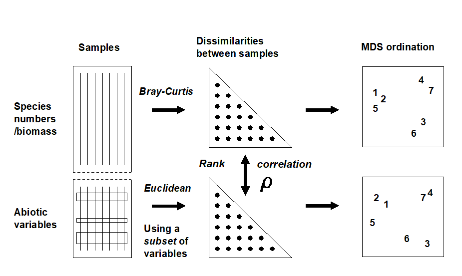
Fig. 11.8. Schematic diagram of the BEST procedure (Bio-Env): selection of the abiotic variable subset maximising rank correlation ($\rho$) between biotic and abiotic (dis)similarity matrices, by checking all combinations of variables.
The BEST (Bio-Env) procedure
The matching of biotic to environmental patterns can now take place ȹ, as outlined schematically in Fig. 11.8. Combinations of the environmental variables are considered at steadily increasing levels of complexity, i.e. k variables at a time (k = 1, 2, 3, ..., v). Table 11.2 displays the outcome for the Exe estuary nematodes.
Table 11.2. Exe estuary nematodes {X}. Combinations of the 6 environmental variables, taken k at a time, yielding the best matches of biotic and abiotic similarity matrices for each k, as measured by weighted Spearman rank correlation $\rho _ s$; bold type indicates overall optimum. See earlier text for variable abbreviations.
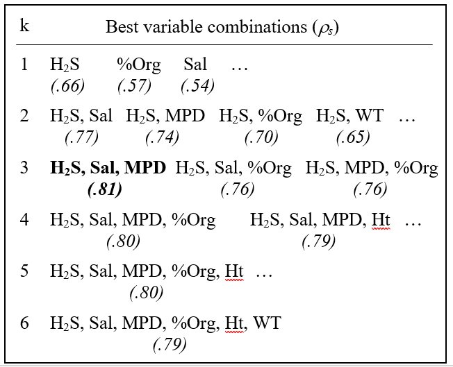
The single abiotic variable which best groups the sites, in a manner consistent with the faunal patterns, is the depth of the $H _ 2 S$ layer ($\rho _ s = 0.66$); next best is the organic content ($\rho _ s = 0.57$), etc. Naturally, since the faunal ordination is not one-dimensional (Fig. 11.7a), it would not be expected that a single abiotic variable would provide a very successful match, though knowledge of the H$_ 2$S variable alone does distinguish points to the left and right of Fig. 11.7a (samples 1 to 4 and 6 to 9 have lower values than for samples 5, 10 and 12 to 19, with sample 11 between).
The best 2-variable combination also involves depth of the $H _ 2 S$ layer but adds the interstitial salinity. The correlation ($\rho _ s = 0.77$) is markedly better than for the single variables, and this is the combination shown in Fig. 11.7b. The best 3-variable combination retains these two but adds the median particle diameter, and gives the overall optimum value for $\rho _ s$ of 0.81 (Fig. 11.7c); $\rho _ s$ drops slightly to 0.80 for the best 4- and higher-way combinations. The results in Table 11.2 do therefore seem to accord with the visual impressions in Fig. 11.7.Ɥ In this case, the first column of Table 11.2 has a hierarchical structure: the best combination at one level is always a subset of the best combination on the line below. This is not guaranteed since all combinations have been evaluated and simply ranked, though it will tend to happen when the explanatory variables are only weakly related to each other, if at all.
An exhaustive search over v variables involves
$$ \sum _ {k =1} ^ {v} = \frac{ v ! } { k ! \left( v - k \right) ! } = 2 ^ v - 1 \tag{11.5} $$
combinations, i.e. 63 for the Exe estuary study, though this number quickly becomes prohibitive when v is larger than about 15. Above that level, one could consider stepwise procedures which search in a more hierarchical fashion, adding and deleting variables one at a time (see the BEST BVStep option, Chapter 16). In practice though, it may be desirable to limit the scale of the search initially, for a number of reasons, e.g. always to include a variable known from previous experience or external information to be potentially causal. Alternatively, scatter plots of the environmental variables may demonstrate that some are highly inter-correlated and nothing in the way of improved ‘explanation’ could be achieved by entering them all into the analysis.
An example is given by the Garroch Head macrofauna study {G}, for which the 11 abiotic variables of Table 11.1 are first transformed, to validate the use of Euclidean distances and standard product-moment correlations (page 11.2). As indicated earlier, choice of transformations is aided by a draftsman plot, i.e. scatter plots of all pairwise combinations of variables, Fig. 11.9. Here, this is after all the concentration variables, but not water depth, have been log transformed℈, in line with the recommendations on page 11.2
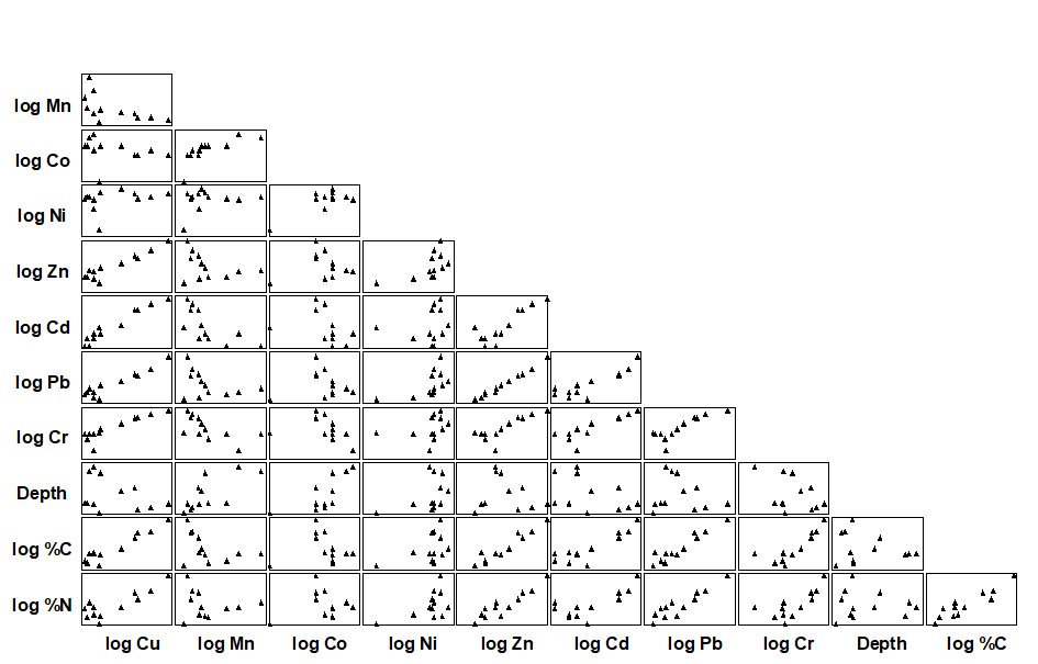
Fig. 11.9. Garroch Head macrofauna {G}. Draftsman plot (all possible pairwise scatter plots) for the 11 abiotic variables recorded at 12 sampling stations across the sewage sludge dumpsite. All variables except water depth have been log transformed.
The draftsman plot, and the associated correlation matrix between all pairs of variables, can then be examined for evidence of collinearity (page 11.3), indicated by straight-line relationships, with little scatter, in Fig. 11.9. A further rule-of-thumb would be to reduce all subsets of (transformed) variables which have mutual correlations averaging more than about 0.95 to a single representative. This suggests that %C, Cu, Zn and Pb are so highly inter-correlated that it would serve no useful purpose to leave them all in the BEST analysis. For every good match that included %C, there would be equally good matches including Cu, Zn or Pb, leading to a plethora of effectively identical solutions. Here, the organic carbon load (%C) is retained and the other three excluded, leaving 8 abiotic variables in the full Bio-Env search. This results in an optimal match of the biotic pattern with %C, %N and Cd ($\rho _ s = 0.86$). The corresponding ordination plots are seen in Fig. 11.10. The biotic MDS of Fig. 11.10a, though structured mainly by a single strong gradient towards the dump centre (e.g. the organic enrichment gradient seen in Fig. 11.10b), is not wholly 1-dimensional. Additional information, on a heavy metal, appears to improve the ‘explanation’.
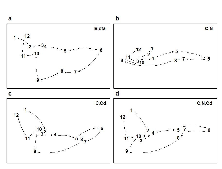
Fig 11.10. Garroch Head macrofauna {G}. MDS plots for the 12 sampling stations across the sewage-sludge dump site (Fig. 8.3), based on: a) species biomass, as in Fig. 11.5a; b)-d) three combinations of carbon, nitrogen and cadmium concentrations (log transformed) in the sediments, the best match with the biota over all combinations of the 8 variables being for %C, %N and Cd ($\rho_s$ = 0.86). (Stress = 0.05, 0, 0.01, 0.01).
Further examples of the Bio-Env procedure are given in
Clarke & Ainsworth (1993)
,
Clarke (1993)
,
Somerfield, Gee & Warwick (1994a)
,
Somerfield, Gee & Warwick (1994b)
and many subsequent applications. For a series of data sets on impacts on benthic macrofauna around N Sea oil rigs,
Olsgard, Somerfield & Carr (1997)
and
Olsgard, Somerfield & Carr (1998)
use the Bio-Env procedure in a particularly interesting way. They examine which transformations (Chapter 9) and what level of taxonomic aggregation (Chapter 10) tend to maximise the Bio-Env correlation, $\rho$. The hypotheses examined are that certain parts of the community, on the spectrum of rare to common species, may delineate the underlying impact gradient more clearly (see page 9.4), as may some taxonomic levels, higher than species (see page 10.1).
Global BEST test
Another question which naturally arises is the extent to which the conclusions from a BEST run can be supported by significance tests. This is problematic given the lack of model assumptions underlying this procedure, which can be seen as both a strength (i.e. generality, ease of understanding, simplicity of interpretation) and a weakness (lack of a structure for formal statistical inference). A simple RELATE test is available (see page 6.10 and later) of the hypothesis that there is no relationship between the biotic information and that from a specified set of abiotic variables, i.e. that $\rho$ is effectively zero. This can be examined by a permutation or randomisation test, of a type met previously on pages 6.8 & 6.10, in which $\rho$ is recomputed for all (or a large random subset of) permutations of the sample labels in one of the two underlying similarity matrices. As usual, if the observed value of $\rho$ exceeds that found in 95% of the simulations, which by definition correspond to unrelated ordinations, then the null hypothesis can be rejected at the 5% level.
Note however that this is not a valid procedure if the abiotic set being tested against the biotic pattern is the result of optimal selection by the BEST procedure, on the same data. For v variables, this is implicitly the same as carrying out $2 ^ v –1$ null hypothesis tests, each of which potentially runs a 5% risk of Type 1 error (rejecting the null hypothesis when it is really true). This rapidly becomes a very large number of tests as v increases, and a naïve RELATE test on the optimal combination is almost certain to indicate a significant biotic-abiotic relation, even with entirely random data sets!
What is needed here is a randomisation test which incorporates the fitting stage and thus allows for the selection bias in the optimal solution. This can be readily achieved, though requires quite a heavy computational load. The requirement is to generate the (null) distribution of the maximum $\rho$ that can be obtained, by an exhaustive search over all subsets of environmental variables (see Fig. 11.8), when there really is no matching structure between biotic and abiotic data. The null situation is again produced by randomly permuting the columns (samples) of one of the data matrices on the left hand side of Fig. 11.8, in relation to the other. The two matrices are then treated as if their samples do have matching labels and the full Bio-Env procedure is applied, to find the subset of environmental variables which gives the ‘best’ match. Of course, this $\rho$ would not be expected to be large, since any real match has been destroyed by the permutation, but $\rho$ will clearly be greater than zero since the largest of all the $2 ^ v –1$ calculated correlations has been selected.
So far, then, we have produced a single value from the null distribution of (max) $\rho$, when there is no biotic-environmental link. This whole procedure is now repeated a total of (say) 999 times, each time randomly reshuffling the columns of the abiotic matrix and running through the entire Bio-Env procedure, to obtain an optimum $\rho$. A histogram of these values is the null distribution, namely, the expected range of BEST Bio-Env $\rho$ values that it is possible to obtain by chance when there is no biotic to abiotic link. As usual, comparison with the observed value of $\rho$ shows the statistical significance, or otherwise, of this observed $\rho$.
Fig 11.11 shows the resulting histograms for the two examples used in this chapter to illustrate the BEST (Bio-Env) procedure. For both the Exe nematodes {X} and the Garroch Head macrofauna {G}, we can be confident in interpreting the biota to environment links because the observed best matches of $\rho _ s$ = 0.81 and 0.86 are larger than could have been obtained by chance: they are greater than any of their 999 simulated $\rho _ s$ values (p<0.1%). Note, however, how far the null distributions are from being centred at $\rho = 0$, particularly for the Garroch Head data, which has a mode at about 0.25 and right-tail values up to about 0.7. This reflects both the small number of sites that are being matched and the simplicity of the strong linear gradient in the sample structure. With 8 abiotic variables (and thus a choice of 255 possible subsets) it is clearly not that difficult to find an environmental combination, by chance, that gives some degree of match to any rank order of the samples along a line.
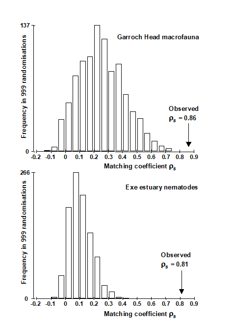
Fig. 11.11. Garroch Head macrofauna {G} and Exe estuary nematodes {X}. Global BEST (Bio-Env) test for a significant relationship between community and environmental samples. The histograms are the null permutation distributions of possible values for the best Bio-Env match (Spearman $\rho_s$), in the absence of a biota-environment relationship.
The same idea can be used to derive a permutation test for the BVStep context, in which only a stepwise-selected set of optimal variables are generated. The simulations of the null condition simply require an equivalent stepwise search on the randomly permuted (and thus non-matching) matrices for the maximum $\rho$, repeated many times to obtain the null distribution for $\rho$. This is the principle of permutation tests: permute the data appropriately to reflect the null condition, then repeat exactly the same steps (however complicated) in calculating the test statistic as were carried out on the data in its original form, and compare the true statistic to the values under permutation.
These tests for Bio-Env and BVStep procedures are together referred to as global BEST tests, and as with the global ANOSIM test of Chaper 6, this becomes an important initial ‘traffic light’. The null hypothesis, of no biotic to abiotic link, must be decisively rejected before any attempt is made to interpret the environmental variables that BEST selects. This is always helped by increasing the number of sites, conditions, times etc that are being matched. For the Exe data, there were 19 sites (compared with 12 for Garroch Head) and only 6 environmental variables, and the null distribution of $\rho _ s$ in Fig. 11.11 now has mode less than 0.1, with right tail values stretching to no higher than about 0.4. Any reasonably large observed $\rho _ s$ is therefore likely to be interpretable.
¶ These might sometimes include biotic as well as abiotic data, e.g. when assessing how coral reef fish communities might be structured by area cover of specific, dominant species of coral.
† Additional reasons for a poor match include: cases where the observed biotic patterns are largely a function of internal stochastic forces, e.g. competitive interactions within the assemblage, rather than external forcing variables; abiotic variables are measured over the wrong spatio-temporal scales in terms of their impact on community structure; there is a large element of random variation from sample to sample, under the same environmental conditions, e.g. the unit sample size is inadequate to characterise the assemblage; and a more technical reason (addressed later) concerning non-additive effects of structuring variables. In all these cases, the procedure may fail to ‘explain’ the community structure well, in terms of the provided set of environmental variables.
§ For example, in spite of the very low stress in Fig. 11.7, a 2-d Procrustes fit of 11.7a with 11.7c will be rather poor, since the (5, 10) and (12–19) groups are interchanged between the plots. Yet, the interpretation of the two analyses is fundamentally the same (five clusters, with the (5, 10) group out on a limb etc). This match will probably be better in 3-d but will be fully expressed, without arbitrary dimensionality constraints, in the underlying similarity matrices.
‡ This matrix correlation statistic has already been met, e.g. on pages 6.8, 6.10, 7.5, and will be used extensively again later.
⸙ This is so defined by Clarke & Ainsworth (1993) because it is algebraically related to the average of the harmonic mean of each ($r _ i $, $s _ i$) pair. The denominator term, $r _ i + s _ i$, down-weights the contribution of large ranks; these are the low similarities, the highest similarity corresponding to the lowest value of rank similarity (1), as usual. Note that $\rho _w$ and $\tau$ tend to give consistently lower values than $\rho _s$ for the same match; nothing should therefore be inferred from a comparison of absolute values of $\rho _s$, $\tau$ and $\rho _w$.
ȹ This is implemented in the PRIMER BEST routine, which includes both a full search (the Bio-Env option) and a sequential, stepwise, form of this (BVStep), when there are too many variables to permit an exhaustive search.
Ɥ This will not always be the case if the 2-d faunal ordination has non-negligible stress. It is the matching of the similarity matrices which is definitive, although it would usually be a good idea to plot the abiotic ordination for the best combination at each value of k, in order to gauge the effect of a small change in $\rho$ on the interpretation. Experience suggests that combinations giving the same value of $\rho$ to two decimal places do not give rise to ordinations which are distinguishable in any practically important way, thus it is recommended that $\rho$ is quoted only to this accuracy, as in Table 11.2.
℈ This actually uses a log(c+x) transformation where c is a constant such as 1 or 0.1. The necessity for this, rather than a simple log(x) transform, comes from the zero values for the Cd concentrations in Table 11.1, log(0) being undefined. A useful rule-of-thumb here is to set the constant c to the lowest non-zero measurement, or the concentration detection limit.