7.6 Example: Garroch Head macrofauna
An example where the biotic sample axis could have sensibly been ordered according to an a priori spatial layout, or in terms of environmental conditions (e.g. the first principal component of a suite of organics and heavy metal levels in sediments, PC1), is that of the root-transformed biomass data from 12 sites on an E-W transect across the sewage-sludge dump-ground in the Firth of Clyde, discussed in Chapter 4, {G}. A shade plot very similar to that of Fig. 7.9a will result from sites ordered by this PC1, and there is again a marked diagonalisation – species turn-over is strong as sites approach the high pollution levels closer to the dump-ground. In fact, we have chosen here to use this instead as an example contrasting the two choices that PRIMER gives for ordering samples. Fig. 7.9a is displayed with a reduced species set (of 35), using a seriation on both site and species axes, unconstrained by dendrograms for either axis. In contrast, Fig. 7.9b shows the result of ordering both sites and species in an order given by a nearest neighbour trajectory.
Nearest neighbour ordering of shade plot axes
Whilst arranging sample and species axes according to serial trends is generally the preferred choice for a shade plot, and is certainly instructive in the current case, there will be situations in which this is not so appropriate, for example if a cyclic pattern of samples is expected or observed (e.g. seasonality, cyclic inter-annual change etc) and the data matrix would then not be expected to diagonalise. In such cases, we may want to place the samples in order of some observed natural trajectory in community structure, not limited to a simple gradient. An illustration of this is in Figs. 7.9c and d, which are the same nMDS plot, for root-transformed biomass at the 12 transect sites (data as in the shade plot above), and Bray-Curtis similarities. It is only the trajectories, defining the axis orders in the otherwise identical shade plots, which differ, with 7.9c showing the optimum serial change and 7.9d an approximate solution to the ‘travelling salesman’ problem. This, as its name suggests, tries to find a route through all the sites, of minimum distance, and starting from whichever point minimises that length. Distance in this context means (Bray-Curtis) sample dissimilarity among the samples, not actual distance in the (only approximate) low-d nMDS ordination. And here there is a fairly natural trajectory joining the sites, which is not the zig-zag route of the serial trend, and the shade plot of 7.9b orders the samples and the species by these attempted minimum trajectories (in the case of the species order, minimisation is of the total index of association along its trajectory).
There is again potentially an immense computational problem here (termed NP-hard in numerical analysis jargon), since there are 12!/2 sample orders and 35!/2 species orders to consider. The solution implemented in PRIMER is a simple, non-iterative routine (which is often surprisingly effective) known as the ‘greedy travelling salesman’ or nearest neighbour ordering, and is simply described. First, join the two sites (say) which have the lowest dissimilarity, then go into a loop in which the nearest neighbour (lowest dissimilarity) to each current end point is found, the lowest of these two values defining the next link in the chain.
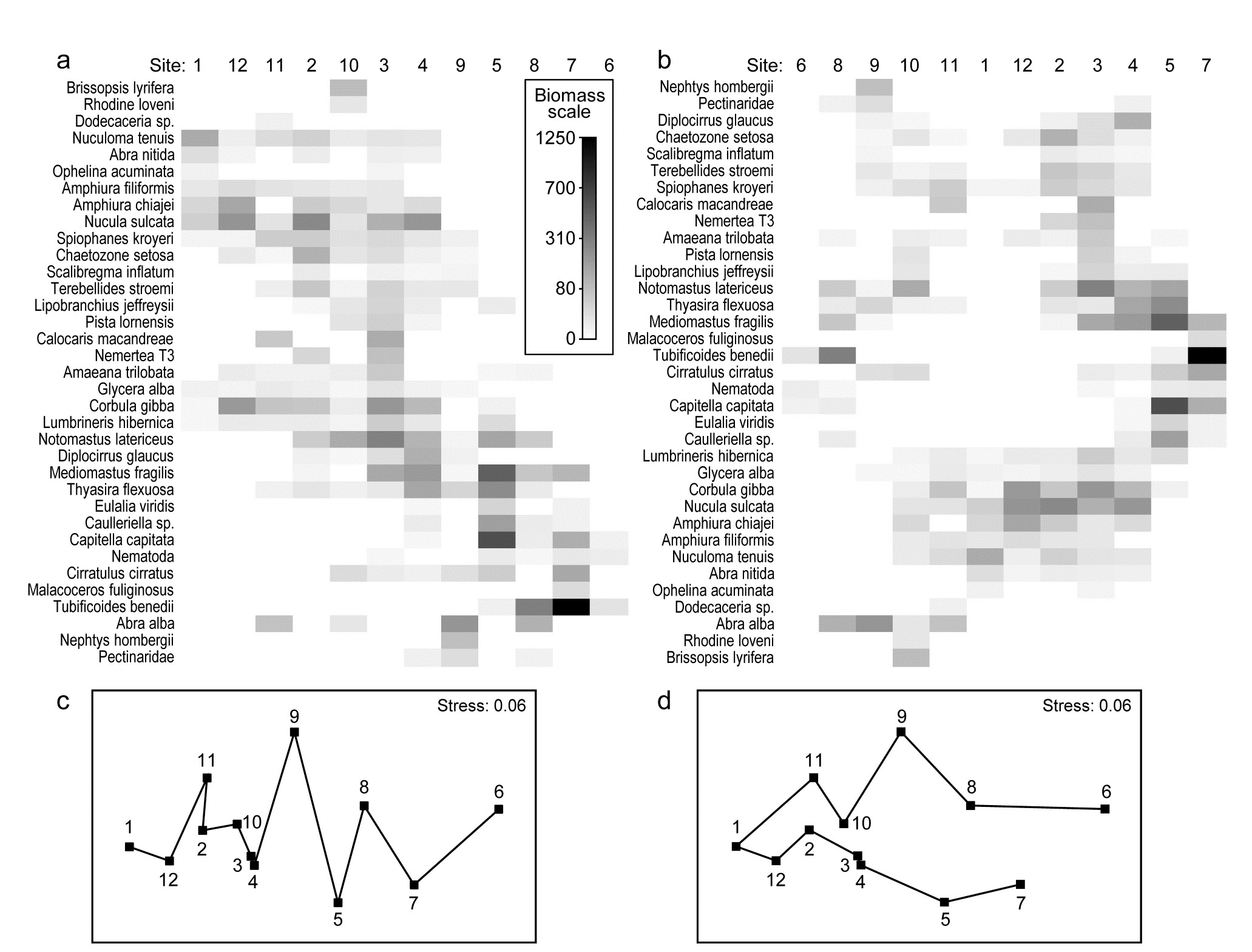
Fig. 7.9. Garroch Head macrofauna {G}. Shade plots of sites 1-12 on an E-W transect (Fig. 1.5) covering a sewage-sludge dumpground (centred at site 6), based on square-root transformed biomass of 35 macrofaunal species, namely those accounting for at least 1% of the total biomass at one or more sites. The grey-scale intensity key has units back-transformed to the original biomass measurements. Axes for samples and species are ordered by: a) iterative maximisation independently on both axes (from 1000 starting configurations) of the seriation statistic, $\rho$, based for samples on Bray-Curtis similarities on root-transformed biomass, and for species on the association index on untransformed but species-standardised data; b) using the same similarity and association measures, both axes independently placed in nearest neighbour order (using the ‘greedy travelling salesman’ algorithm). Neither axis, on either plot, is constrained to be a rotation of a cluster dendrogram. The nMDS plot of the 12 sites (on the Bray-Curtis similarities) is shown with: c) serial and d) nearest neighbour trajectories from the sample orders in (a) and (b) respectively.
The process thus works outwards from the first join, adding points at one or other end of the trajectory (or even all at the same end), until all samples are linked. The procedure is the same for species, the only arbitrariness remaining being the same as for seriation, viz. whether the shade plot samples are ordered from left to right or vice-versa (and the species top to bottom or vice-versa); PRIMER simply allows a ‘flip’ option on both axes to suit the user’s preference.
We return to seriation of the sample and species axes to make one interesting final point about shade plots. The previous, clear-cut, examples may have given the impression that it is easy to see sample patterns in the data matrix using a shade plot, in whatever form the matrix is entered, but this is rarely the case – the key step is an effective grouping or ordering of the axes.
¶ Note that this nearest neighbour trajectory is not the same thing as the minimum spanning tree (MST) met in point 4 on page 5.3. That is a more tractable problem and has an efficient algorithm for a precise solution, Gower & Ross (1969) , the key difference being that the MST allows branching (see Fig. 5.3b). Of course, this is not helpful in the current context of needing a 1-d ordering of the samples or species.