15.2 Meta-analysis of marine macrobenthos

This method was initially devised as a means of comparing the severity of community stress between various cases of both anthropogenic and natural disturbance. On initial consideration, measures of community degradation which are independent of the taxonomic identity of the species involved would be most appropriate for such comparative studies. Species composition varies so much from place to place depending on local environmental conditions that any general species-dependent response to stress would be masked by this variability. However, diversity measures are also sensitive to changes in natural environmental variables and an unperturbed community in one locality could easily have the same diversity as a perturbed community in another. Also, to obtain comparative data on species diversity requires a highly skilled and painstaking analysis of species and a high degree of standardisation with respect to the degree of taxonomic rigour applied to the sample analysis; e.g. it is not valid to compare diversity at one site where one taxon is designated as Nematodes with another at which this taxon has been divided into species.

The problem of natural variability in species composition from place to place can be potentially overcome by working at taxonomic levels higher than species. The taxonomic composition of natural communities tends to become increasingly similar at these higher levels. Although two communities may have no species in common, they will almost certainly comprise the same phyla. For soft-bottom marine benthos, we have already seen in Chapter 10 that disturbance effects are detectable with multivariate methods often at the highest taxonomic levels, even in some instances where these effects are rather subtle and are not evidenced in univariate measures even at the species level, e.g. the Ekofisk {E} study.
 

Meta-analysis is a term widely used in biomedical statistics and refers to the combined analysis of a range of individual case-studies which in themselves are of limited value but in combination provide a more global insight into the problem under investigation. Warwick & Clarke (1993a) have combined macrobenthic data aggregated to phyla from a range of case studies {J} relating to varying types of disturbance, and also from sites which are regarded as unaffected by such perturbations. A choice was made of the most ecologically meaningful units in which to work, bearing in mind the fact that abundance is a rather poor measure of such relevance, biomass is better and production is perhaps the most relevant of all (Chapter 13). Of course, no studies have measured production (P) of all species within a community, but many studies provide both abundance (A) and biomass (B) data. Production was therefore approximated using the allometric equation:

$$ P = (B/A) ^ {0.73} \times A \tag{15.1} $$

where B/A is simply the mean body-weight, and 0.73 is the average exponent of the regression of annual production on body-size for macrobenthic invertebrates. Since the data from each study are standardised (i.e. production of each phylum is expressed as a proportion of the total) the intercept of this regression is irrelevant. For each data set the abundance and biomass data were first aggregated to phyla, following the classification of Howson (1987) ; 14 phyla were encountered overall (see the later Table 15.1). Abundance and biomass were then combined to form a production matrix using the above formula. All data sets were then merged into a single production matrix and an MDS performed on the standardised, 4th root-transformed data using the Bray-Curtis similarity measure. All macrobenthic studies from a single region (the NE Atlantic shelf) for which both abundance and biomass data were available were used, as follows:

1. A transect of 12 stations sampled in 1983 on a west-east transect (Fig. 1.5) across a sewage sludge dump-ground at Garroch Head, Firth of Clyde, Scotland {G}. Stations in the middle of the transect show clear signs of gross pollution.
    

2. A time series of samples from 1963–1973 at two stations (sites 34 and 2, Fig. 1.3) in West Scottish sea-lochs, L. Linnhe and L. Eil {L}, covering the period of commissioning of a pulp-mill. The later years show increasing pollution effects on the macrofauna, except that in 1973 a recovery was noted in L. Linnhe following a decrease in pollution loading.
    

3. Samples collected at six stations in Frierfjord (Oslofjord), Norway {F}. The stations (Fig. 1.1) were ranked in order of increasing stress A–G–E–D–B–C, based on thirteen different criteria. The macrofauna at stations B, C and D were considered to be influenced by seasonal anoxia in the deeper basins of the fjord.
    

4. Amoco-Cadiz oil spill, Bay of Morlaix {A}. In order not to swamp the analysis with one study, the 21 sampling times have been aggregated into 5 years for the meta-analysis: 1977 = pre-spill year, 1978 = post-spill year and 1979-81 = ‘recovery’ period.
    

5. Two stations in the Skagerrak at depths of 100 and 300m. The 300m station showed signs of disturbance attributable to the dominance of the sediment reworking bivalve Abra nitida.
    

6. An undisturbed station off the coast of Northumberland, NE England.
    

7. An undisturbed station in Carmarthen Bay, S Wales.
    

8. An undisturbed station in Kiel Bay; mean of 22 sets of samples.
    

In all, this gave a total of 50 samples, the disturbance status of which has been assessed by a variety of different methods including univariate indices, dominance plots, ABC curves, measured contaminant levels etc. The MDS for all samples (Fig.15.1) takes the form of a wedge with the pointed end to the right and the wide end to the left. It is immediately apparent that the long axis of the configuration represents a scale of disturbance, with the most disturbed samples to the right and the undisturbed samples to the left. (The reason for the spread of sites on the vertical axis is less obvious). The relative positions of samples on the horizontal axis can thus be used as a measure of the relative severity of disturbance. Another gratifying feature of this plot is that in all cases increasing levels of disturbance result in a shift in the same direction, i.e. to the right. For visual clarity, the samples from individual case studies are plotted in Fig. 15.2, with the remaining samples represented as dots.

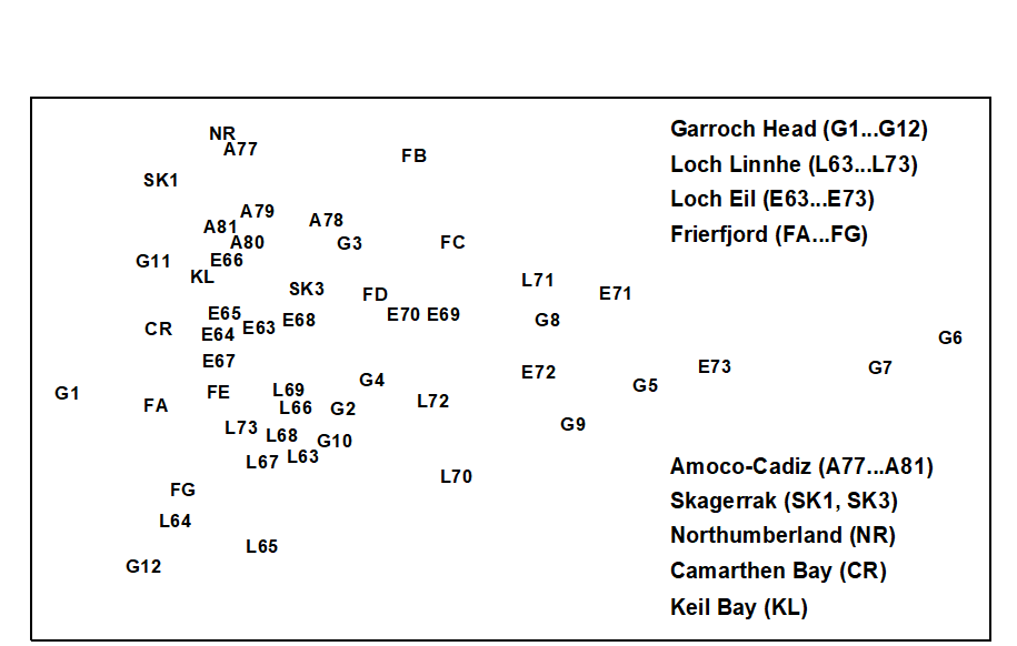
Fig. 15.1. Joint NE Atlantic shelf studies (‘meta-analysis’) {J}. Two dimensional MDS ordination of phylum level ‘production’ data (stress = 0.16).
 

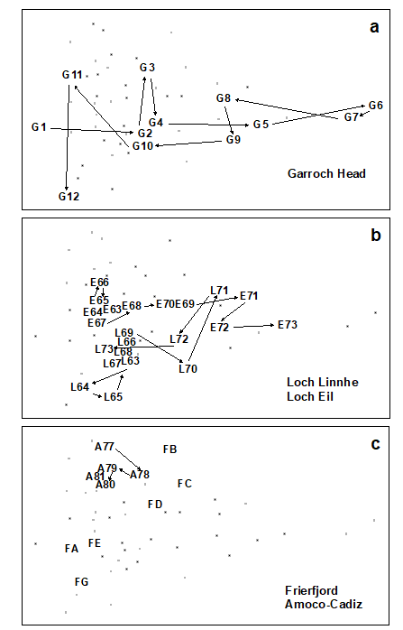
Fig. 15.2. Joint NE Atlantic shelf studies (‘meta-analysis’) {J}. As Fig. 15.1 but with individual studies highlighted: a) Garroch Head (Clyde) dump-ground; b) Loch Linnhe and Loch Eil; c) Frierfjord and Amoco-Cadiz spill (Morlaix).
 

1. Garroch Head (Clyde) sludge dump-ground {G}. Samples taken along this transect span the full scale of the long axis of the configuration (Fig. 15.2a). Stations at the two extremities of the transect (1 and 12) are at the extreme left of the wedge, and stations close to the dump centre (6) are at the extreme right.
    

2. Loch Linnhe and Loch Eil {L}. In the early years (1963–68) both stations are situated at the unpolluted left-hand end of the configuration (Fig. 15.2b). After this the L. Eil station moves towards the right, and at the end of the sampling period (1973) it is close to the right-hand end; only the sites at the centre of the Clyde dump-site are more polluted. The L. Linnhe station is rather less affected and the previously mentioned recovery in 1973 is evidenced by the return to the left-hand end of the wedge.
    

3. Frierfjord (Oslofjord) {F}. The left to right order of stations in the meta-analysis is A–G–E–D–B–C (Fig. 15.2c), exactly matching the ranking in order of increasing stress. Note that the three stations affected by seasonal anoxia (B,C and D) are well to the right of the other three, but are not as severely disturbed as the organically enriched sites in 1) and 2) above.
    

4. Amoco-Cadiz spill, Morlaix {A}. Note the shift to the right between 1977 (pre-spill) and 1978 (post-spill), and the subsequent return to the left in 1979–81 (Fig. 15.2c). However, the shift is relatively small, suggesting that this is only a mild effect.
    

5. Skagerrak. The biologically disturbed 300m station is well to the right of the undisturbed 100m station, although the former is still quite close to the left-hand end of the wedge.
    

6. to 8 Unpolluted sites. The Northumberland, Carmarthen Bay and Keil Bay stations are all situated at the left-hand end of the wedge.

An initial premise of this method was that, at the phylum level, the taxonomic composition of communities is relatively less affected by natural environmental variables than by pollution or disturbance (Chapter 10). To examine this, Warwick & Clarke (1993a) superimposed symbols scaled in size according to the values of the two most important environmental variables considered to influence community structure, sediment grain size and water depth, onto the meta-analysis MDS configuration (a technique described in Chapter 11). Both variables had high and low values scattered arbitrarily across the configuration, which supports the original assumption.

With respect to individual phyla, annelids comprise a high proportion of the total ‘production’ at the polluted end of the wedge, with a decrease at the least polluted sites. Molluscs are also present at all sites, except the two most polluted, and have increasingly higher dominance towards the non-polluted end of the wedge. Echinoderms are even more concentrated at the non-polluted end, with some tendency for higher dominance at the bottom of the configuration (Fig. 15.3a). Crustacea are again concentrated to the left, but this time entirely confined to the top part of the configuration (Fig. 15.3b). Clearly, the differences in relative proportions of crustaceans and echinoderms are largely responsible for the vertical spread of samples at this end of the wedge, but these differences cannot be explained in terms of the effects of any recorded natural environmental variables. Nematoda are clearly more important at the polluted end of the wedge, an obvious consequence of the fact that species associated with organic enrichment tend to be very large in comparison with their normal meiofaunal counterparts (e.g. Oncholaimids), and are therefore retained on the macrofaunal ecologists’ sieves. Other less important phyla show no clear distribution pattern, except that most are absent from the extreme right-hand samples.

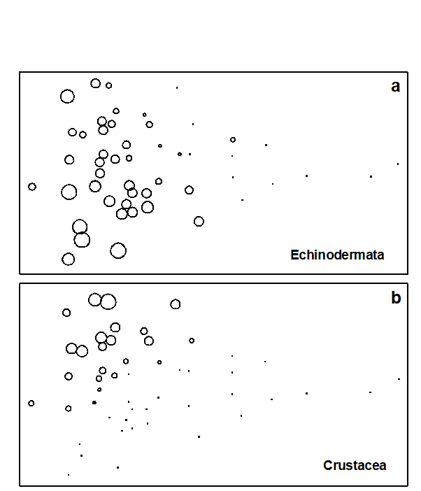
Fig. 15.3. Joint NE Atlantic shelf studies (‘meta-analysis’) {J}. As Fig. 15.1 but highlighting the role of specific phyla in shaping the MDS; symbol size represents % production in each sample from: a) echinoderms, b) crustaceans.

This multivariate approach to the comparative scaling of benthic community responses to environmental stress seems to be more satisfactory than taxon-independent methods, having both generality and consistency of behaviour. It is difficult to assess the sensitivity of the technique because data on abundance and biomass of phyla are not available for any really low-level or subtle perturbations. However, its ability to detect the deleterious effect of the Amoco-Cadiz oil spill, where diversity was not impaired, and to rank the Frierfjord samples correctly with respect to levels of stress which had been determined by a wide variety of more time-consuming species-level techniques, suggests that this approach may retain much of the sensitivity of multivariate methods. It certainly seems, at least, that there is a high signal/noise ratio in the sense that natural environmental variation does not affect the communities at this phyletic level to an extent which masks the response to perturbation. The fact that this meta-analysis ‘works’ has a rather weak theoretical basis. Why should Mollusca as a phylum be more* sensitive to perturbation than Annelida, for example? The answer to this is unlikely to be straightforward and would need to be addressed by considering a broad range of toxicological, physiological and ecological characteristics which are more consistent within than between phyla.

The application of these findings to the evaluation of data from new situations requires that both abundance and biomass data are available. The scale of perturbation is determined by the 50 samples present in the meta-analysis. These can be regarded as the training set against which the status of new samples can be judged. The best way to achieve this would be to merge the new data with the training set to generate a single production matrix for a re-run of the MDS analysis. The positions of the new data in the two dimensional configuration, especially their location on the principal axis, can then be noted. Of course the positions of the samples in the training set may then be altered relative to each other, though such re-adjustments would be expected to be small. It is also natural, at least in some cases, that each new data set should add to the body of knowledge represented in the meta-analysis, by becoming part of an expanded training set against which further data are assessed. This approach would preserve the theoretical superiority and practical robustness of applying MDS (Chapter 5) in preference to ordination methods such as PCA.

However, there are circumstances in which more approximate methods might be appropriate, such as when it is preferable to leave the training data set unmodified. Fortunately, because of the relatively low dimensionality of the multivariate space (14 phyla, of which only half are of significance), a two-dimensional PCA of the ‘production’ data gives a plot which is rather close to the MDS solution. The eigenvectors for the first three principal components, which explain 72% of the total variation, are given in Table 15.1. The value of the PC1 score for any existing or new sample can then easily be calculated from the first column of this table, without the need to re-analyse the full data set. This score could, with certain caveats (see below), be interpreted as a disturbance index. This index is on a continuous scale but, on the basis of the training data set given here, samples with a score of >+1 can be regarded as grossly disturbed, those with a value between –0.2 and +1 as showing some evidence of disturbance and those with values <–0.2 as not signalling disturbance with this methodology. A more robust, though less incisive, interpretation would place less reliance on the absolute location of samples on the MDS or PCA plots and emphasise the movement (to the right) of putatively impacted samples relative to appropriate controls. For a new study, the spread of sample positions in the meta-analysis allows one to scale the importance of observed changes, in the context of differences between control and impacted samples for the training set.

Table 15.1. Joint NE Atlantic shelf studies (‘meta-analysis’) {J}. Eigenvectors for the first three principal components from covariance-based PCA of standardised and 4th root-transformed phylum ‘production’ (all samples).

Phylum	PC1	PC2	PC3
Cnidaria	-0.039	0.094	0.039
Platyhelminthes	-0.016	0.026	-0.105
Nemertea	0.169	0.026	0.061
Nematoda	0.349	-0.127	-0.166
Priapulida	-0.019	0.010	0.003
Sipuncula	-0.156	0.217	0.105
Annelida	0.266	0.109	-0.042
Chelicerata	-0.004	0.013	-0.001
Crustacea	0.265	0.864	-0.289
Mollusca	-0.445	-0.007	0.768
Phoronida	-0.009	0.005	0.008
Echinodermata	-0.693	-0.404	-0.514
Hemichordata	-0.062	-0.067	-0.078
Chordata	-0.012	0.037	-0.003

It should be noted that the training data is unlikely to be fully representative of all types of perturbation that could be encountered. For example, in Fig. 15.1, all the grossly polluted samples involve organic enrichment of some kind, which is conducive to the occurrence of the large nematodes which play some part in the positioning of these samples at the extreme right of the meta-analysis MDS or PCA. This may not happen with communities subjected to toxic chemical contamination only. Also, the training data are only from the NE European shelf, although data from a tropical locality (Trinidad, West Indies) have also been shown to conform with the same trend ( Agard, Gobin & Warwick (1993) ). Other studies have looked at specific impact data merged with the above training set (e.g. Somerfield, Atkins, Bolam et al. (2006) , on dredged-material disposal in UK waters), though these studies have been rather few in number. It is unclear whether this represents a paucity of data of the right type (biomass measurements are still uncommon, in spite of the relative ease with which they can be made, given the faunal sorting necessary for abundance quantification), or reflects a failure of the analysis to generalise.