7.1 Species clustering
Chapter 2 (page 2.4) describes how the original data matrix can be used to define similarities between every pair of species; two species are positively associated (i.e. ‘similar’) if their numbers or biomass or cover etc tend to fluctuate in proportion across samples. They are negatively associated (i.e. ‘dissimilar’) if species have opposite patterns of abundance over samples, with the maximum dissimilarity of 100 occurring if two species are never found in the same samples. Clearly, differences in total abundance of species across samples are of no relevance to association – some species (perhaps with much smaller body size) inevitably have higher counts than others, but can still be perfectly associated with them – so some means of ‘relativising’ species is essential. Pearson correlation does this by dividing by standard deviations and non-parametric correlation by converting to ranks but both are poor measures of species association because of the ‘joint absence’ issue: two species are not similar because neither appear at a particular site or time, yet correlation will make them so. In contrast, standardising species across samples (dividing by their total and multiplying by 100, making species add to 100), followed by Bray-Curtis similarity on pairs of species is not a function of joint absences and takes values over a scale of 0 (perfect ‘negative’ association) to 100 (perfect positive association). It is helpful here to retain the idea of ‘negative’ and ‘positive’ relations even though the index is always in the range (0,100). This combination of species-standardising and Bray-Curtis is more succinctly referred to as Whittaker’s index of association ( Whittaker (1952) ), e.g. of species 1 and 2:
$$ IA = 100 \left[ 1 - \frac{1}{2} \sum_ {j=1} ^n \left|\frac{y_{1j}}{\sum_ {k=1} ^n y _ {1k} } - \frac{y _ {2j}}{\sum_ {k=1} ^n y _ {2k} }\right| \right] \tag{7.1} $$
where $y_{ij}$ is the abundance of the ith species (i=1,.., p) in the jth sample (j=1,.., n).
The species similarity matrix which results can be input to a cluster analysis or ordination in exactly the same way as for sample similarities. This is referred to historically (e.g. see
Field, Clarke & Warwick (1982)
) as inverse or r-mode analysis. However, an ordination is rarely a good idea except in special circumstances with small numbers of species, all of which are well-represented. More typically, there are many species found in small numbers rather randomly across the set of samples, and these have associations to each other which are wildly varying, between 0 (if their few individuals are from different samples) and close to 100 (e.g. if their individuals happen to occur in the same one or two samples). Minor species such as this have very little influence on a samples analysis because their effect on the Bray-Curtis similarities are generally small, but they can provide a large amount of ‘noise’ in a species ordination, resulting in very high stress, and therefore unhelpful displays. An important initial step in most species analyses is therefore to eliminate the ‘rare’ species, e.g. selecting only species which are ‘important somewhere’ in the sense that they account for more than a threshold q% (perhaps q = 1% to 5%) of the total abundance in one or more samples, or by adjusting that percentage to reduce the matrix to a specified number of species n, or by retaining only species which are seen in at least n samples.
Example: Exe estuary nematodes
Fig. 7.1 displays the results of a cluster analysis on the Exe estuary nematode data {X} first seen in Chapter 5, in which 19 intertidal sites with differing environments were sampled bimonthly over a year and time-averaged to give a matrix of 19 samples $\times$ 174 species. Initial species reduction retained only those accounting for ≥5% of the total (averaged) abundance at one or more of the sites, and the index of association was calculated among those 52 species, followed by standard agglomerative hierarchical clustering. From the range of y axis values it is clear that some species are highly positively associated, and other species subsets are negatively associated, apparently found at quite different sites (from the zero associations) but this immediately raises the question as to how much of this clustering structure we are entitled to interpret. The solution to that will be an extension to the SIMPROF procedure first met in Chapter 3 (page 3.5), but this time applied to species rather than sample groupings.
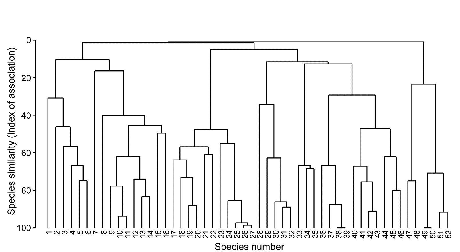
Fig. 7.1. Exe estuary nematodes {X}. Dendrogram using group average linking on species similarities defined by the index of association (i.e. Bray-Curtis on species-standardised but otherwise untransformed abundance for pairs of species compared across the 19 sites). Analysis is only for the species accounting for ≥5% of the total abundance at one or more of the sites (the 52 species numbers are defined later, in Fig. 7.7).