7.5 Example: Bristol Channel zooplankton
This example, last seen in Chapter 3, consists of 24 (seasonally-averaged) zooplankton net samples at 57 sites in the Bristol Channel, UK. Fig. 7.8 shows the shade plot for fourth-root transformed abundances. All 24 species are used and this is again an example where there was no specific a priori structure to the samples, so various clustering methods were used in Figs. 3.9 and 3.10 to group the samples (with Type 1 SIMPROF tests), and for the hierarchical methods it is appropriate to display dendrograms on both axes. The species axis again uses the index of association among untransformed species counts and agglomerative clustering, this time without the SIMPROF tests (Type 3) and, purely to demonstrate that any method of clustering can be used on either axis, the sample grouping utilises the unconstrained divisive algorithm of the PRIMER UNCTREE routine, Fig. 3.9, based on a maximisation of the (ANOSIM) R statistic on each binary split. The 4 significantly different groups of sites given by SIMPROF tests are again shown by vertical lines and (in spite of the heavy transform) the grouping can now be seen to be driven by a very few dominant species, perhaps no more than 8 or 9 of the 24 species, which clearly typify the four clusters and discriminate them from each other. It can also readily be appreciated why two alternative methods, seen in Fig. 3.10 (standard agglomerative and k-R clustering), which again give just four groups, differ in respect of only the allocation of three sites: 9, 23 and 24. For example, the trade-off between absence (or nearly so) of Eurytemora, Temora sp. and Centropages hamatus decides the placement of sites 9 and 24 in groups A or B, and the high values for the Calanus and Paracalanus species mitigate against a move of 23 to B.
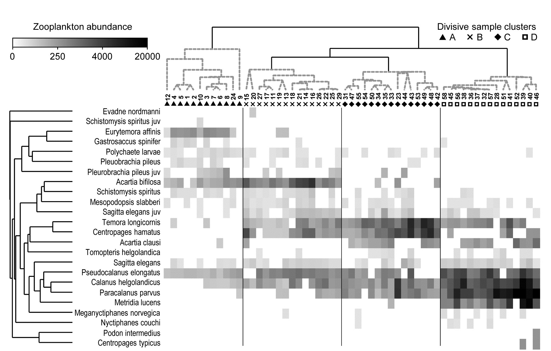
Fig. 7.8. Bristol Channel zooplankton {B}. Shade plot of abundance (averaged over seasons) of 24 zooplankton species from 57 sites, with linear grey-scale intensity proportional to fourth-root abundance (see the key for back-transform to original abundances). Sites have been grouped using Bray-Curtis similarities on the transformed data, by hierarchical, unconstrained divisive clustering (UNCTREE), as in Fig. 3.9, together with (Type 1) SIMPROF tests which identify four groups, A-D in Fig. 3.10b. The dendrogram is further rotated to produce a site ordering which optimises the matrix correlation $\rho$ with a serial model (gradient of community change). Species are also clustered, this time with the standard agglomerative method, based on ‘index of association’ resemblances computed on species-standardised (but otherwise untransformed) abundances; their dendrogram is again rotated to maximise the seriation statistic $\rho$, non-parametrically correlating their resemblances to the distance structure of a linear sequence.
Serial ordering of shade plot axes
This example is not just about grouping however. The MDS plots of Fig. 3.10 have already demonstrated that the rather clear clustering of sites forms part of a gradation of community change (and this is clearly associated with, if not actually driven by, the salinity gradient, 3.10b). The shade plot routine in PRIMER also incorporates a powerful facility which attempts to re-order either (or both) of the samples and species axes, independently of each other, in such a way as to maximise the serial change in the similarity pattern over the final ordering(s). In keeping with the non-parametric philosophy of other core techniques, this utilises the RELATE $\rho$ statistic, which will be used frequently in later chapters, but which was first met in equation (6.3) and discussed in terms of measuring serial change on page 6.10, on the ordered ANOSIM test. This is a non-parametric Mantel-type statistic, computing a rank correlation coefficient (for example Spearman’s $\rho$) between matching entries of two dissimilarity/distance matrices, namely the resemblance matrix (e.g. Bray-Curtis dissimilarity of the biological samples) and distances among points equi-spaced on a line (so that neighbouring points are one step apart, next-but-one neighbours are two steps apart, etc). We need to ‘run before we can walk’ here because later we discuss more straightforward RELATE examples, in which the community samples are tested for how much simple seriation they show in their transect or time order of collection, i.e. tested against known a priori ordering of the samples in space or time (or environmental condition). In the current context, we are not using $\rho$ as a test statistic at all, but simply as a useful way of measuring the degree of serial change in a resemblance matrix, for any given ordering of its rows (and columns)¶.
In theory, we could envisage looking at all possible sample orderings, calculating the $\rho$ seriation statistic for each, and choosing the order that maximises $\rho$. This is not viable however (there are 57!/2 possible orders, i.e. 2$ \times 10^{76}$) and an iterative search procedure is required, to attempt to get close to the optimum $\rho$. As with previous search procedures (such as for MDS ordination), the iterative process can converge to a solution which is some way from the optimal one, so repeat runs are required (1000 are suggested, if this runs in a reasonable time), from randomly different starting orders, and the best selected.†
This is still an intensive search problem however, and there are limitations which this unconstrained search procedure would ignore here, namely that we wish to display a dendrogram along the sample axis, showing the clustering (and here, the SIMPROF groups). The vast majority of the permutations of sample ordering would conflict with that hierarchy. Chapter 3 described the arbitrariness in ordering of a dendrogram and how it was not to interpreted as an ordination – but it is not completely arbitrary. The clustering and sub-clustering structures must be maintained, and the plot is determined only down to random rotation of the bars of the ‘mobile’ it can be considered to represent (i.e. with horizontal lines as bars and vertical lines as strings). So a constrained seriation of the samples is required in this case, iteratively searching through the set of possible rotations of the dendrogram for that which again gets as close as possible to optimising the seriation statistic $\rho$. This is a further option in the PRIMER shade plot routine and is the ordering seen in Fig. 7.8. In fact, the reduction in the immense size of the search space that this constraint induces does seem to make the algorithm more efficient, and good orderings will often result with a much smaller degree of computation.
Exactly the same constrained seriation procedure is also implemented on the species axis of Fig. 7.8, this time using the species resemblance matrix (index of association measure) §. The ability to seriate one or other (or both) axes imparts an order and structure to the data matrix which can often be apparent in the multivariate analysis – here in the strong gradient of samples (Fig. 3.10b) as well as the group structure – but which can be difficult to spot in the matrix itself without such rearrangement of rows and columns. (A striking example of this is seen later, in Fig. 7.10).
It is important to note that these orderings are carried out independently for samples and species, if both are performed. The sample re-arrangement uses only the sample similarities, and the species ordering is quite immaterial to the calculation of those resemblances. In the same way, species similarities make no use of the sample ordering, and they are all that is used in the clustering or seriation of the species. Now, if both axes are rearranged to be as close to a serial trend as possible then it is inevitable that the matrix will have at least a very weak diagonalisation‡, even if what is being seriated is just ‘noise’ rather than real ‘signal’. So visual evidence of diagonalisation of the matrix is not, in itself, conclusive evidence of a trend in the samples – that comes from a RELATE ($\rho$) seriation test on the sample similarities, mentioned earlier. In other words, shade plots are not tools for testing but for interpretation of structures established by testing.
However, in other cases, where the sample axis is in a fixed order based on spatial location or a time course – or the result of seriation of samples on independent information such as environmental conditions – then apparent diagonalisation of the shade plot, after the species have been seriated, does become prima facie evidence of a real gradient of community structure in that sample order. This is formally established by a seriation test on the sample resemblances, in rank correlation with (distances from) that sample order.
¶ This is analogous to the way we used the ANOSIM R statistic in the binary divisive and k-R clustering methods of Chapter 3, in which a test of the null hypothesis R=0 (as in ANOSIM) would have been quite incorrect, and irrelevant. What was needed there was, for example, to find a binary division of a cluster which maximised the value of ANOSIM R between the two sub-clusters formed by this division. Here we use RELATE $\rho$ in the same way, to find an ordering of the samples which maximises the match of their dissimilarities to a triangular matrix of distances among equi-spaced points along a line. This is showing us the ‘natural order’ in which the samples would align themselves, in terms of their community change, if no external constraints were made.
†This unconstrained seriation search, on either axis, is one of the options in the PRIMER Shade Plot routine. That it may not find the exact maximum $\rho$ of the $2 \times 10 ^ {76}$ possibilities is not a concern. We are not seeking the ‘correct’ solution but trying to display samples (and species) in a reasonably natural order, which will enhance the prospects for visual interpretation of the data matrix.
§ Note that the latter is computed by first species-standardising the untransformed data, not standardising the fourth-root transformed values represented by the grey-scale rectangles. This is true for the Exe example above and all other shade plots in this manual, though species-standardising transformed abundances could certainly be considered in some situations (for the reasons discussed in point 3 on page 7.3). Note that it is also universally true in these examples that the sample clustering or seriation is performed on the sample resemblances calculated from the full set of species, not the reduced set of species that it is convenient to view in a shade plot (though in the case of Fig. 7.8 there is no need to reduce to a smaller number of species). In a particular context, it might make sense to use only the reduced species set for all aspects of the sample analysis (and of course this is easy to do in PRIMER) but the difference this would make to multivariate analyses will typically be inconsequential, and it is logically more satisfactory to cluster and seriate the samples in the shade plot using the full set of species, which are the basis of the MDS plots, ANOSIM and RELATE tests etc. This is certainly the path which PRIMER’s Wizard for Matrix display assumes will be needed, though the direct Shade plot routine permits wide flexibility.
‡ This interesting and powerful independence of seriation on the two axes is in contrast to Correspondence Analysis-based tools, which produce a 2-way table by iteratively reweighting the axes in turn, so that the converged solution forces a mutual ordering to optimise diagonalisation. Here the diagonalisation emerges more spontaneously, and may not be guaranteed in cases of extreme species turnover. For example, if a group of samples has a completely disjunct species set from all other samples, those samples and species will be placed at one or other end of their respective gradients, but at which end is entirely arbitrary, the similarities (or associations) to all other samples (or species) being zero. In such extreme cases, it might be thought neater to follow automatic seriation by manual rotation of a disassociated group to a more ‘natural’ place. The ability to manually rotate dendrograms by clicking on ‘bars’ in the usual way is built into the PRIMER Shade Plot routine.