16.5 Second-stage MDS
It is not normally a viable sampling strategy, for soft-sediment benthos at least, to use BVStep to identify a subset of species as the only ones whose abundance is recorded in future, since all specimens have to be sorted and identified to species, to determine the subset. Saving of monitoring effort on identification can sometimes be made, however, by working at a higher taxonomic level than species (see Chapter 10). Where full species-based information is available, MDS plots can be generated at different levels of taxonomic aggregation (i.e. using species, genera, families, etc) and the configurations visually compared. Another axis of choice for the biologist is that of the transformation applied to the original counts (or biomass/cover etc). Chapter 9 shows that different transformations pick out different components of the assemblage, from only the dominant species (no transform), through increasing contributions from mid-abundance and less-common species ($\sqrt{}$, $\sqrt{} \sqrt{}$, log) to a weighting placing substantial attention on less-common species (presence/absence). The environmental impact, or other spatial or temporal ‘signal’, may be clearer to discern from the ‘noise’ under some transformations than it is for others.
Amoco-Cadiz oil spill
The difficulty arises that so many MDS plots can be produced by these choices that visual comparison is no longer easy, and it is always subjective, relying only on the 2-d approximation in an MDS plot, rather than the full high-dimensional information. For example, Fig. 16.4 displays the MDS plots for the Morlaix study at only two taxonomic levels: data at species and aggregated to family level, for each of the full range of transformations, but it is already difficult to form a clear summary of the relative effects of the different choices. However, part of the solution to this problem has already been met earlier in the chapter. For every pair of MDS plots – or rather the similarity matrices that underlie them – it is easy to define a measure of how closely the sample patterns match: it is the Spearman rank correlation ($\rho$) applied to the elements of the similarity matrices. Different transformations and aggregation levels will affect the absolute range of calculated Bray-Curtis similarities but, as always, it is their relative values that matter. If all statements of the form ‘sample A is closer to B than it is to C’ are identical for the two similarity matrices then the conclusions of the analyses will be identical, the MDS plots will match perfectly and $\rho$ will take the value 1.
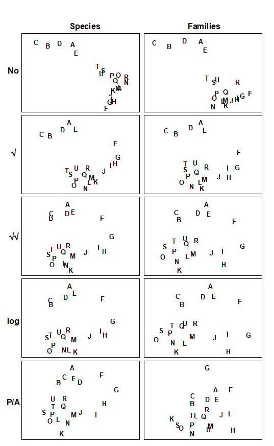
Fig. 16.4. Amoco-Cadiz oil spill {A}. MDS plots of the 21 sampling occasions (A, B, C, …) in the Bay of Morlaix, for all macrobenthic species (left) and aggregated into families (right), and for different transformations of the abundances (in top to bottom order: no transform, root, 4th-root, log(1+x), presence/absence). For precise dates see the legend to Fig. 10.4; the oil-spill occurred between E and F (stress, reading left to right: 0.06, 0.07; 0.07, 0.08; 0.09, 0.10; 0.09, 0.09; 0.14, 0.18).
Table 16.3 shows the results of calculating the rank correlations ($\rho$) between every pair of analysis options represented in Fig. 16.4. For example, the largest correlation is 0.996 for untransformed species and family-level analyses, the smallest is 0.639 between untransformed and presence/absence family-level analyses, etc. Though Table 16.3 is clearly a more quantitatively objective description of the pairwise comparisons between analyses, the plethora of coefficients still make it difficult to extract the overall message. Looking at the triangular form of the table, however, the reader can perhaps guess what the next step is! Spearman correlations are themselves a type of similarity measure: two analyses telling essentially the same story have a higher $\rho$ (high similarity) than two analyses giving very different pictures (low $\rho$, low similarity). All that needs adjustment is the similarity scale, since correlations can potentially take values in (–1, 1) rather than (0,100) say. In practice, negative correlations in this context will be rare (but if they arise they indicate even less similarity of the two pictures) but the problem is entirely solved anyway by working, as usual, with the ranks of the $\rho$ values, i.e. rank (dis)similarities. It is then natural to input these into an MDS ordination, as shown schematically in Fig. 16.5.
Table 16.3. Amoco-Cadiz oil spill {A}. Spearman correlation matrix between every pair of similarity matrices underlying the 10 plots of Fig. 16.4, measuring the extent to which they ‘tell the same story’ about the 21 Morlaix samples. These correlations (rank ordered) are treated like a similarity matrix and input to a second-stage MDS. Key: s = species-level analysis, f = family-level; 0 = no transform, 1 = root, 2 = 4th root, 3 = log(1+x), 4 = presence /absence.
| s0 | s1 | s2 | s3 | s4 | f0 | f1 | f2 | f3 | |
|---|---|---|---|---|---|---|---|---|---|
| s1 | .970 | ||||||||
| s2 | .862 | .949 | |||||||
| s3 | .852 | .942 | .995 | ||||||
| s4 | .736 | .847 | .961 | .946 | |||||
| f0 | .996 | .965 | .855 | .845 | .726 | ||||
| f1 | .949 | .993 | .961 | .958 | .865 | .947 | |||
| f2 | .791 | .893 | .972 | .974 | .953 | .785 | .924 | ||
| f3 | .760 | .869 | .962 | .971 | .946 | .753 | .904 | .993 | |
| f4 | .645 | .756 | .877 | .870 | .923 | .639 | .792 | .946 | .929 |
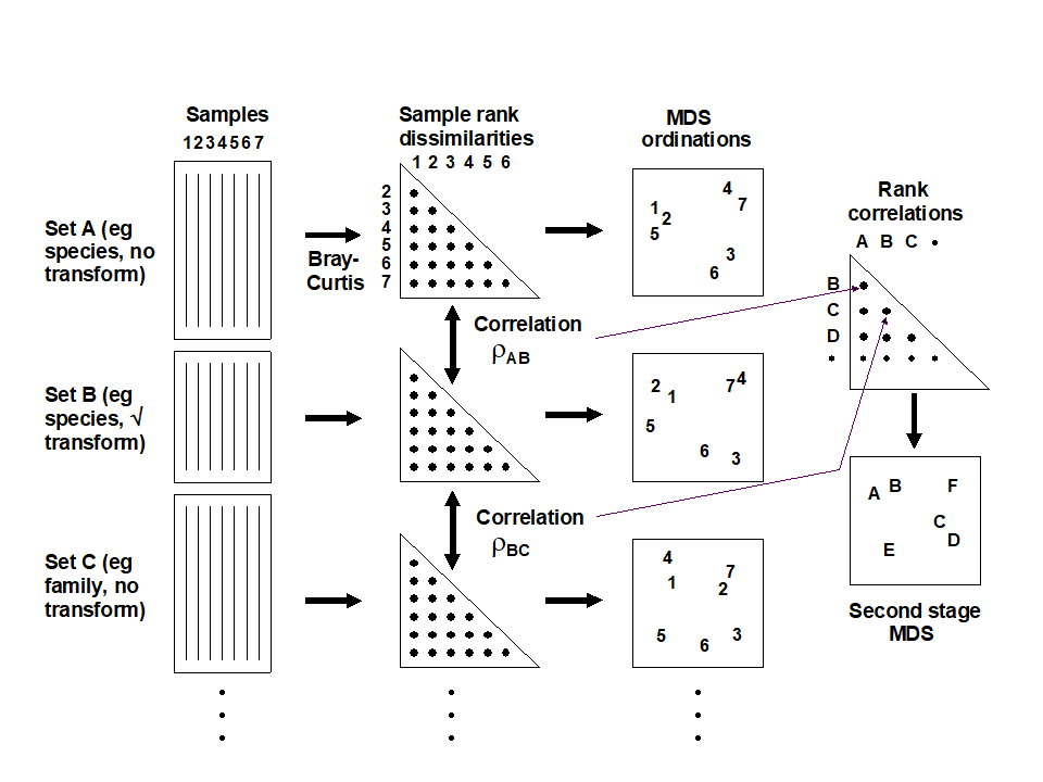
Fig. 16.5. Schematic diagram of the stages in quantifying and displaying agreement, by second-stage MDS, of different multivariate analyses of a corresponding set of samples.
The resulting picture is termed a second-stage MDS and is displayed in Fig. 16.6 for the Morlaix analyses of Fig. 16.4. The relationship between the various analysis options is now summarised in a clear and straightforward fashion (with near-zero stress). The different transformations form the main (left to right) axis, in steady progression through: no transform, $\sqrt{}$, $\sqrt{}\sqrt{}$ and log(1+x), to pres/abs. The difference between species and family level analyses largely forms the other (bottom to top) axis. Three important points are immediately clear:
-
Log and $\sqrt{}\sqrt{}$ transforms are virtually identical in their effect on the data, with differences between these transformations being much smaller than that between species and family-level analyses in that case.
-
With the exception of these two, the transformations generally have a much more marked effect on the outcome than the aggregation level (the relative distance apart on the MDS of the points representing different transformations, but the same taxonomic level, is much greater than the distance apart of species and family-level analyses, for the same transformation).
-
The effect of taxonomic aggregation becomes greater as the transformation becomes more severe, so that for presence/absence data the difference between species and family-level is much more important than it is for untransformed or mildly transformed counts. Whilst this is not unexpected, it does indicate the necessity to think about analysis choices in combination, when designing a study.
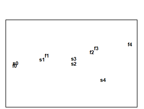
Fig. 16.6. Amoco-Cadiz oil spill {A}. Second-stage MDS of the 10 analyses of Fig. 16.4. The proximity of the points indicates the extent to which different analysis options capture the same information. s = species-level analysis, f = family-level; 0 = no transform, 1 = root, 2 = 4th root, 3 = log(1+x), 4 = presence /absence. Stress = 0.01, so the 2-d picture tells the whole story, e.g. that choice of aggregation level has less effect here than transformation. .
Other applications
The concept of a second-stage MDS used on rank correlations between similarity matrices – from different taxonomic aggregation levels (species, genus, family, trophic group) and, in the same analysis, different faunal groups (nematodes, macrofauna) recorded for the same set of sites – was introduced by Somerfield & Clarke (1995) , for studies in Liverpool Bay and the Fal estuary, UK. Olsgard, Somerfield & Carr (1997) and Olsgard, Somerfield & Carr (1998) expanded the scope to include the effects of different transformation, simultaneously with differing aggregation levels, for data from N Sea oilfield studies.¶ Other interesting applications include Kendall & Widdicombe (1999) who examined different body-size components of the fauna as well as different faunal groups, from a hierarchical spatial sampling design (spacings of 50cm, 5m, 50m, 500m) in Plymouth subtidal waters. They used a second-stage MDS to display the effects of different combinations of body-sizes, faunal groups and transformation. Olsgard & Somerfield (2000) introduced the pattern from environmental variables as an additional point on a second-stage MDS, together with biotic analyses from different faunal components (polychaetes, molluscs, crustacea, echinoderms) at another N Sea oilfield. The idea is that biotic subsets whose multivariate pattern links well to the environmental data will be represented by points on the second-stage MDS which lie close to the environmental point. The converse operation can also be envisaged, as a visual counterpart to the Bio–Env procedure. For small numbers of environmental variables, the abiotic patterns from subsets of these can be represented as points on the second-stage MDS, in which the (fixed) biotic similarity matrix is also shown. The best environmental combinations should then ‘converge’ on the (single) biotic point.
¶ They also carried out another interesting analysis, assessing Bio–Env results in the light of analysis choices. It was hypothesised earlier (pages 9.4 and 10.1), that a contaminant impact may manifest itself more clearly in the assemblage pattern for intermediate transform and aggregation choices. Olsgard, Somerfield & Carr (1997) do indeed show, for the Valhall oilfield, that the Bio–Env matching of sediment macrobenthos to the degree of disturbance from drilling muds disposal (measured by sediment THC, Ba concentrations etc), was optimised by intermediate transform ($\sqrt{}$) and aggregation level (family).