3.2 Hierarchical agglomerative clustering
The most commonly used clustering techniques are the hierarchical agglomerative methods. These usually take a similarity matrix as their starting point and successively fuse the samples into groups and the groups into larger clusters, starting with the highest mutual similarities then lowering the similarity level at which groups are formed, ending when all samples are in a single cluster. Hierarchical divisive methods perform the opposite sequence, starting with a single cluster and splitting it to form successively smaller groups.
The result of a hierarchical clustering is represented by a tree diagram or dendrogram, with the x axis representing the full set of samples and the y axis defining a similarity level at which two samples or groups are considered to have fused. There is no firm convention for which way up the dendrogram should be portrayed (increasing or decreasing y axis values) or even whether the tree can be placed on its side; all three possibilities can be found in this manual.
Fig. 3.1 shows a dendrogram for the similarity matrix from the Frierfjord macrofauna, a subset of which is in Table 3.1. It can be seen that all four replicates from sites A, D, E and G fuse with each other to form distinct site groups before they amalgamate with samples from any other site; that, conversely, site B and C replicates are not distinguished, and that A, E and G do not link to B, C and D until quite low levels of between-group similarities are reached.
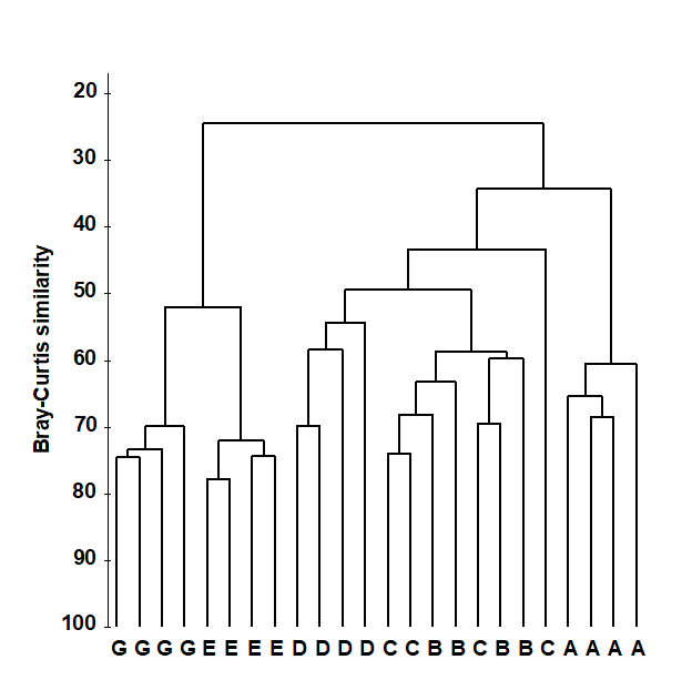
Fig. 3.1. Frierfjord macrofauna counts {F}. Dendrogram for hierarchical clustering (using group-average linking) of four replicate samples from each of sites A-E, G, based on the Bray- Curtis similarity matrix shown (in part) in Table 3.1.
The mechanism by which Fig. 3.1 is extracted from the similarity matrix, including the various options for defining what is meant by the similarity of two groups of samples, is best described for a simpler example.
Construction of dendrogram
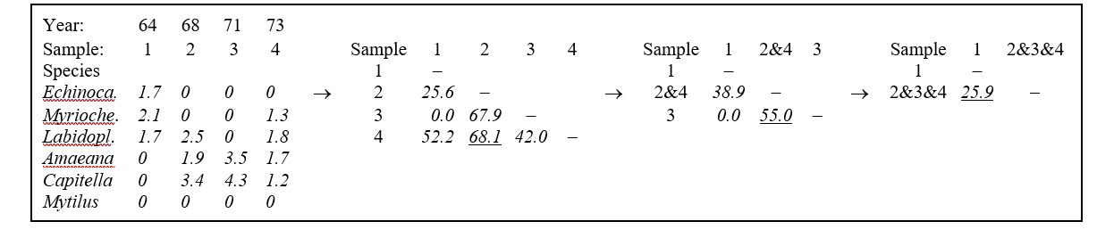
Table 3.2 shows the steps in the successive fusing of samples, for the subset of Loch Linnhe macrofaunal abundances used as an example in the previous chapter. The data matrix has been $\sqrt{}\sqrt{}$-transformed, and the first triangular array is the Bray-Curtis similarity of Table 2.2.
Samples 2 and 4 are seen to have the highest similarity (underlined) so they are combined, at similarity level 68.1%. (Above this level there are considered to be four clusters, simply the four separate samples.) A new similarity matrix is then computed, now containing three clusters: 1, 2&4 and 3. The similarity between cluster 1 and cluster 3 is unchanged at 0.0 of course but what is an appropriate definition of similarity S(1, 2&4) between clusters 1 and 2&4, for example? This will be some function of the similarities S(1,2), between samples 1 and 2, and S(1,4), between 1 and 4; there are three main possibilities here.
a) Single linkage. S(1, 2&4) is the maximum of S(1, 2) and S(1, 4), i.e. 52.2%.
b) Complete linkage. S(1, 2&4) is the minimum of S(1, 2) and S(1, 4), i.e. 25.6%.
c) Group-average link. S(1, 2&4) is the average of S(1, 2) and S(1, 4), i.e. 38.9%.
Table 3.2 adopts group-average linking, hence
$$ S(2 \& 4, 3) = \left[ S(2, 3) + S(4, 3) \right]/2 = 55.0 $$
The new matrix is again examined for the highest similarity, defining the next fusing; here this is between 2&4 and 3, at similarity level 55.0%. The matrix is again reformed for the two new clusters 1 and 2&3&4 and there is only a single similarity, S(1, 2&3&4), to define. For group-average linking, this is the mean of S(1, 2&4) and S(1, 3) but it must be a weighted mean, allowing for the fact that there are twice as many samples in cluster 2&4 as in cluster 3. Here:
$$ S(1, 2 \& 3 \& 4) = \left[ 2 \times S (1, 2 \& 4) + 1 \times S(1, 3) \right]/3 = \left[ 2 \times 38.9 + 1 \times 0 \right]/3 = 25.9 $$
Table 3.2. Loch Linnhe macrofauna {L} subset. Abundance array after $\sqrt{}\sqrt{}$-transformation, the resulting Bray-Curtis similarity matrix and the successively fused similarity matrices from a hierarchical clustering, using group average linking.
Though it is computationally efficient to form each successive similarity matrix by taking weighted averages of the similarities in the previous matrix (known as combinatorial computation), an alternative which is entirely equivalent, and perhaps conceptually simpler, is to define the similarity between the two groups as the simple (unweighted) average of all between-group similarities in the initial triangular matrix (hence the terminology Unweighted Pair Group Method with Arithmetic mean, UPGMA¶). So:
$$ S(1, 2 \& 3 \& 4) = \left[S(1, 2) + S(1, 3) + S(1, 4)\right]/3 = (25.6 + 0.0 + 52.2)/3 = 25.9,$$
the same answer as above.
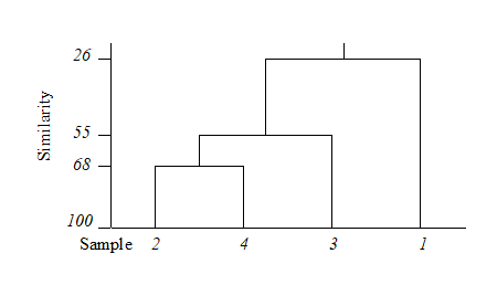
The final merge of all samples into a single group therefore takes place at similarity level 25.9%, and the clustering process for the group-average linking shown in Table 3.2 can be displayed in the following dendrogram.
Dendrogram features
This example raises a number of more general points about the use and appearance of dendrograms.
-
Samples need to be re-ordered along the x axis, for clear presentation of the dendrogram; it is always possible to arrange samples in such an order that none of the dendrogram branches cross each other.
-
The resulting order of samples on the x axis is not unique. A simple analogy would be with an artist’s ‘mobile’; the vertical lines are strings and the horizontal lines rigid bars. When the structure is suspended by the top string, the bars can rotate freely, generating many possible re-arrangements of samples on the x axis. For example, in the above figure, samples 2 and 4 could switch places (new sequence 4, 2, 3, 1) or sample 1 move to the opposite side of the diagram (new sequence 1, 2, 4, 3), but a sequence such as 1, 2, 3, 4 is not possible. It follows that to use the x axis sequence as an ordering of samples is misleading.
-
Cluster analysis attempts to group samples into discrete clusters, not display their inter-relations on a continuous scale; the latter is the province of ordination and this would be preferable for the simple example above. Clustering imposes a rather arbitrary grouping on what appears to be a continuum of change from an unpolluted year (1964), through steadily increasing impact (loss of some species, increase in abundance of opportunists such as Capitella), to the start of a reversion to an improved condition in 1973. Of course it is unwise and unnecessary to attempt serious interpretation of such a small subset of data but, even so, the equivalent MDS ordination for this subset (met in Chapter 5) contrasts well with the relatively unhelpful information in the above dendrogram.
-
The hierarchical nature of this clustering procedure dictates that, once a sample is grouped with others, it will never be separated from them in a later stage of the process. Thus, early borderline decisions which may be somewhat arbitrary are perpetuated through the analysis and may sometimes have a significant effect on the shape of the final dendrogram. For example, similarities S(2, 3) and S(2, 4) above are very nearly equal. Had S(2, 3) been just greater than S(2, 4), rather than the other way round, the final picture would have been a little different. In fact, the reader can verify that had S(1, 4) been around 56% (say), the same marginal shift in the values of S(2, 4) and S(2, 3) would have had radical consequences, the final dendrogram now grouping 2 with 3 and 1 with 4 before these two groups come together in a single cluster. From being the first to be joined, samples 2 and 4 now only link up at the final step. Such situations are certain to arise if, as here, one is trying to force what is essentially a steadily changing pattern into discrete clusters.
Dissimilarities
Exactly the converse operations are needed when clustering from a dissimilarity rather than a similarity matrix. The two samples or groups with the lowest dissimilarity at each stage are fused. The single linkage definition of dissimilarity of two groups is the minimum dissimilarity over all pairs of samples between groups; complete linkage selects the maximum dissimilarity and group-average linking involves just an unweighted mean dissimilarity.
Linkage options
The differing consequences of the three linkage options presented earlier† are most easily seen for the special case used in Chapter 2, where there are only two species (rows) in the original data matrix. Samples are then points in the species space, with the (x,y) axes representing abundances of (Sp.1, Sp.2) respectively. Consider also the case where dissimilarity between two samples is defined simply as their (Euclidean) distance apart in this plot.
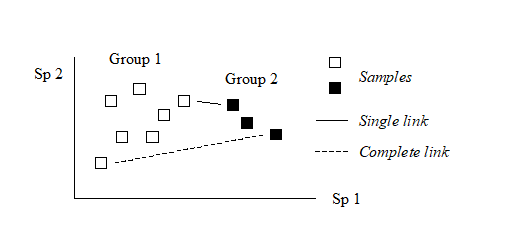
In the above diagram, the single link dissimilarity between Groups 1 and 2 is then simply the minimum distance apart of the two groups, giving rise to an alternative name for the single linkage, namely nearest neighbour clustering. Complete linkage dissimilarity is clearly the maximum distance apart of any two samples in the different groups, namely furthest neighbour clustering. Group-average dissimilarity is the mean distance apart of the two groups, averaging over all between-group pairs.
Single and complete linkage have some attractive theoretical properties. For example, they are effectively non-metric. Suppose that the Bray-Curtis (say) similarities in the original triangular matrix are replaced by their ranks, i.e. the highest similarity is given the value 1, the next highest 2, down to the lowest similarity with rank n(n–1)/2 for n samples. Then a single (or complete) link clustering of the ranked matrix will have the exactly the same structure as that based on the original similarities (though the y axis similarity scale in the dendrogram will be transformed in some non-linear way). This is a desirable feature since the precise similarity values will not often have any direct significance; what matters is their relationship to each other and any non-linear (monotonic) rescaling of the similarities would ideally not affect the analysis. This is also the stance taken for the preferred ordination technique in this manual’s strategy, the method of non-metric multi-dimensional scaling (MDS, see Chapter 5).
However, in practice, single link clustering has a tendency to produce chains of linked samples, with each successive stage just adding another single sample onto a large group. Complete linkage will tend to have the opposite effect, with an emphasis on small clusters at the early stages. (These characteristics can be reproduced by experimenting with the special case above, generating nearest and furthest neighbours in a 2-dimensional species space). Group-averaging, on the other hand, is often found empirically to strike a balance in which a moderate number of medium-sized clusters are produced, and only grouped together at a later stage.
¶ The terminology is inevitably a little confusing therefore! UPGMA is an unweighted mean of the original (dis)similarities among samples but this gives a weighted average among group dissimilarities from the previous merges. Conversely, WPGMA (also known as McQuitty linkage) is defined as an unweighted average of group dissimilarities, leading to a weighted average of the original sample dissimilarities (hence WPGMA).
† PRIMER v7 offers single, complete and group average linking, but also the flexible beta method of Lance & Williams (1967) , in which the dissimilarity of a group (C) to two merged groups (A and B) is defined as $\delta _ {C,AB} = (1 – \beta)[(\delta _ {CA} + \delta _ {CB} ) / 2] + \beta \delta _ {AB} $. If $\beta = 0$ this is WPGMA, $( \delta _ {CA} + \delta _ {CB} ) / 2$, the unweighted average of the two group dissimilarities. Only negative values of $\beta$, in the range (-1, 0), make much sense in theory; Lance and Williams suggest $ \beta = -0.25 $ (for which the flexible beta has affinities with Gower’s median method) but PRIMER computes a range of $ \beta$ values and chooses that which maximises the cophenetic correlation. The latter is a Pearson matrix correlation between original dissimilarity and the (vertical) distance through a dendrogram between the corresponding pair of samples; a dendrogram is a good representation of the dissimilarity matrix if cophenetic correlation is close to 1. Matrix correlation is a concept used in many later chapters, first defined on page 6.10, though there (and usually) with a Spearman rank correlation; however the Pearson matrix correlation is available in PRIMER 7’s RELATE routine, and can be carried out on the cophenetic distance matrix available from CLUSTER. (It is also listed in the results window from a CLUSTER run). In practice, judged on the cophenetic criterion, an optimum flexible beta solution is usually inferior to group average linkage (perhaps as a result of its failure to weight $\delta _ {CA}$ and $\delta _ {CB}$ appropriately when averaging ‘noisy’ data).