5.10 Example: Messolongi lagoon diatoms

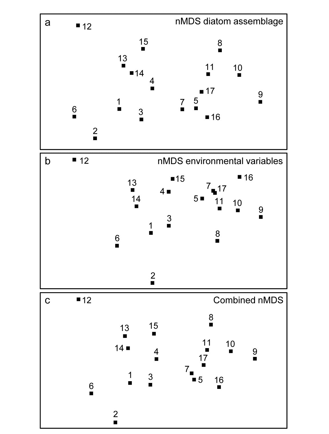
Danielidis (1991) sampled 17 lagoons in E Central Greece for diatom communities (193 species), and also recorded a suite of 12 water-column variables: temperature, salinity, DO$_2$, pH, PO$_4$, total P, NH$_3$, NO$_2$, NO$_3$, inorganic N and SiO$_2$. After global square root transformations and Bray-Curtis dissimilarities are calculated on the species densities, and selective log transforms (of the nutrients) and Euclidean distances are calculated on the environmental variables, Fig. 5.14a&b display the resulting separate nMDS ordinations. In this case, there is a remarkable degree of uniformity in the way these two independent sets of variables describe the sample patterns, suggesting that the structuring environmental variables for these communities have been correctly identified (and this idea leads into the BEST technique in Chapter 11 for further refinement of ‘structuring variable’ selection). A combined nMDS of the two resemblance matrices is given in Fig. 5.14c. The 2-d stress of 0.13, c.f. 0.09 and 0.08 for the separate biotic and abiotic plots, shows that one must expect an increased stress even when agreement is very good.

Fig. 5.14. Messolongi diatoms {m}. nMDS plots for17 lagoon sites based on: a) 193 species (from Bray-Curtis dissimilarities), b) 12 water-column variables (normalised Euclidean distances), c) combined nMDS, the configuration simultaneously minimising average stress from the biotic and abiotic Shepard diagrams. Stress: a) 0.09, b) 0.08, c) 0.13.