9.5 Dispersion weighting
There is a clear dichotomy, in defining sample similarities, between methods which give each variable (species) equal weight, such as normalisation or species standardisation, and those which treat counts (of whatever species) as comparable and therefore give greater weight to more numerically dominant species. As pointed out above, giving rare species the same weight as dominant ones bundles in a great deal of ‘noise’, diffusing the ‘signal’, but it can be equally unhelpful to allow the analysis to be driven by highly abundant, but very erratic counts, from motile species occurring in schools, or more static species which are spatially clumped by virtue of their colonising or reproductive patterns. A severe transformation will certainly reduce the dominance of such species, but it can be seen as rather a blunt instrument, since it also squeezes out much of the quantitative information from mid- or low-abundance species, some of which may not exhibit this erratic behaviour over replicates of the same condition (site/time/treatment), because they are not spatially clumped. If data are genuinely counts and information from replicates is available, a better solution ( Clarke, Chapman, Somerfield et al. (2006) ) is to weight species differently, according to the reliability of the information they contain, namely the extent to which their counts in replicates display overdispersion.
It is important to appreciate the subtlety of the idea of dispersion weighting: species are not down-weighted because they show large variation across the full set of samples; they may do that because their abundance changes strongly across the different conditions (and it is precisely those species which will best indicate community change). Species are down-weighted if they have high variability, for their mean count, in replicates of the same condition. In fact, we must be careful to make no use of information about the way abundances vary across conditions when determining the weight each species gets in the analysis, otherwise we are in serious danger of a self-fulfilling argument (e.g. high weight given to species which, on visual inspection, appear to show the greatest differences between groups will clearly bias tests unfairly in favour of demonstrating community change, just as surely as picking out only a subset of species, a posteriori, to input to the analyses).
Dispersion weighting (DW) therefore simply divides all counts for a single species by a particular constant, calculated as the index of dispersion D (the ratio of the variance to the mean) within each group, averaged across all groups to give divisor $\overline{D}$ for that species. The justification for this is a rather simple but general model in which counts of a species in each replicate are from a generalised Poisson distribution. Details are given in Clarke, Chapman, Somerfield et al. (2006) , but the concept is illustrated in Fig. 9.2, thought of as replicate quadrats ‘catching’ a different number of centres of population (clumps) for that species as the conditions (groups) change, but with each centre containing a variable number of individuals, with unknown probability distribution. The only assumption is that the different conditions change the number of clumps but not the average or standard deviation of the clump size, e.g. in some sites a particular species is quite commonly found and in others hardly at all, but its propensity to school or clump is something innate to the species.
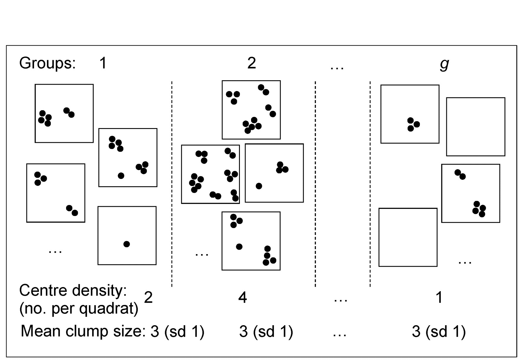
Fig 9.2 Simple graphic of generalised Poisson model for counts of a single species: centres of population are spatially random but with density varying across groups (sites/times/treatments). The distribution of the number of individuals(≥1) found at each centre is assumed constant across groups, though unknown.
Technically, for a particular species, if the number of centres in a replicate from group g has a Poisson distribution with mean $\nu _ g$ and the number of individuals at each centre has an unknown distribution with mean $\mu$ and variance $\sigma^2$, then $X _ j$, the count in the jth replicate from group g, has mean $\nu _ g \mu$ and variance $\nu _ g (\mu ^ 2 + \sigma ^ 2)$. Thus the index of dispersion D, the ratio of variance to mean counts for the group is $(\mu ^ 2 + \sigma ^ 2)/\mu$ and this is not a function of $\nu _ g$, i.e. D is the same for all groups, and an average D can be computed across groups (weighted, if replicates unbalanced). Dividing all counts by this average gives values which have the ‘Poisson-like’ property of variance $\approx$ mean.
The process is repeated for all species separately. Note that there is certainly no assumption that the clump size distribution is the same for all species, not even in distributional form: some species will be heavily clumped, others not at all, with all possibilities in between, but all are reduced by DW to giving (non-integral) abundances that are equally variable in relation to their mean, i.e. the unwanted contributions made by large but highly erratic counts are greatly down-weighted by their large dispersion indices.
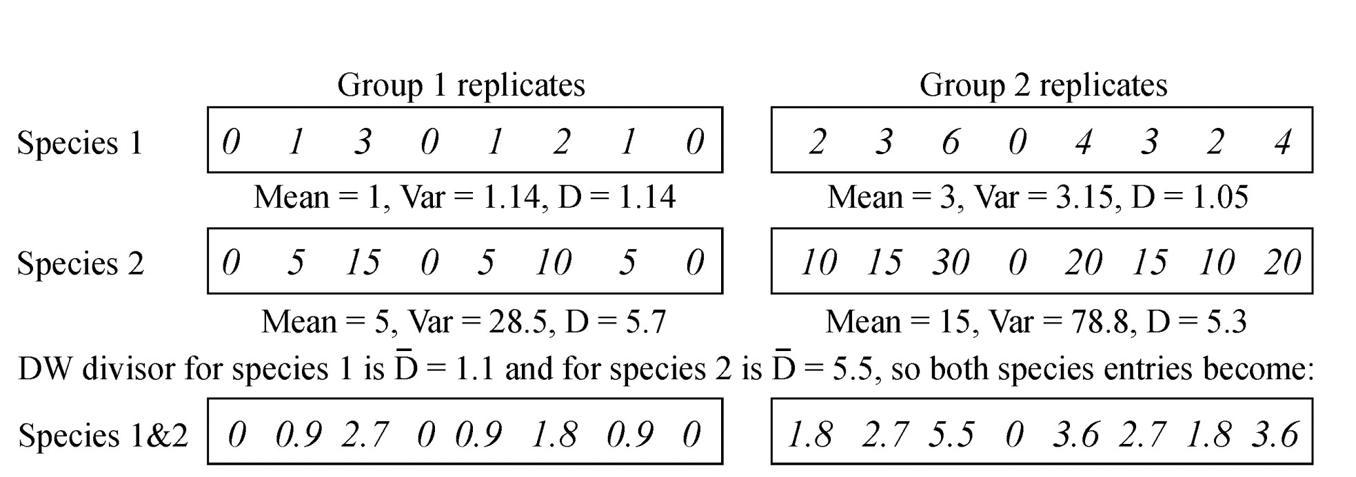
Table 9.5. Simple example of dispersion weighting (DW) on abundances from a matrix of two species sampled for two groups (e.g. sites/times), each of eight replicates. Prior to DW, species 2 would receive greater weight but its arrivals are clumped. After DW, the species have identical entries in the matrix.
One simple (over-simple) way of thinking of this is that we count clumps instead of individuals, and the calculation for such a simple hypothetical case is illustrated above. Here, there are two groups, with 8 replicates per group and two species. The individuals of species 1 arrive independently (the replicates show the Poisson-like property of variance $\approx$ mean) whereas species 2 has an identical pattern of arrivals but of clumps of 5 individuals at a time. Dividing through each set of species counts by the averaged dispersion indices (1.1 and 5.5 respectively) would reduce both rows of data to the same Poisson-like ‘abundances’.¶
However, DW is much more general than this simple case implies. The generalised Poisson model certainly includes the case of fixed-size clumps, and the even simpler case where the clump size is one, so that individuals arrive into the sample independently of each other, for which the counts are then Poisson and D=1 (DW applies no down-weighting). More realistically, it includes the Negative Binomial distribution as a special case, a distribution often advocated for fully parametric modelling of overdispersed counts (e.g. recently by Warton, Wright & Wang (2012) ). Such modelling needs the further assumption that the clump size distribution is of the same type for all species, namely Fisher’s log series. Also subsumed under DW are the Neyman type A (where the clump size distribution is also Poisson) and the Pólya-Aeppli (geometric clump size distribution) and many others.
Our approach here is to remain firmly distribution-free. In order to remove the large contributions that highly erratic (clumped) species counts can make to multivariate analyses such as the SIMPER procedure, it is not necessary (as Warton, Wright & Wang (2012) advocate) to throw out all the advantages of a fully multivariate approach to analysis, based on a biologically relevant similarity matrix, replacing them with what might be characterised as ‘parallel univariate analyses’. (This seems a classic case of ‘throwing the baby out with the bathwater’). Instead, it is simply necessary first to down-weight such species semi-parametrically, by dispersion weighting, which subsumes the negative binomial and many other commonly-used parametric models for overdispersed counts, and the (perceived§) problem disappears.
¶ In fact the counts for species 1 would not lead to rejection of the null hypothesis of independent random arrivals (D=1) in this case, using the permutation test discussed later, so no DW would be applied to species 1.
§ It is relevant to point out here that the later example (and much other experience) suggests that, whilst DW is more logically satisfactory than the cruder use of severe transformations for this purpose, the practical differences between analyses based on DW and on simple transforms are, at their greatest, only marginal. Since most of the 10,000+ papers using PRIMER software in its 20-year history have used transformed data (PRIMER even issues a warning if Bray-Curtis calculation has not been preceded by a transformation), Warton’s conclusions, largely based on analyses of untransformed data, that “hundreds of papers every year currently use methods [which] risk undesirable consequences” seem unjustified.