2.6 More on resemblance measures
On the grounds that it is better to walk before you try running, discussion of comparisons between specific similarity, dissimilarity and distance coefficients, that the PRIMER software refers to generally by the term resemblance measures, is left until after presentation of a useful suite of multivariate analyses that can be generated from a given set of sample resemblances, and then how such sets of resemblances themselves can be compared (second-stage analysis, Chapter 16). One topic can realistically be addressed here, though.
Missing data and resemblance calculation
Missing data in this context does not mean missing whole samples (e.g. the intention was to collect five replicates but at one location only four were taken). The latter is better described as unbalanced sampling design and is handled automatically, and without difficulty, by most of the methods in this manual (an exception is when trying to link the biotic assemblage at a site to a set of measured environmental variables, e.g. in the BEST routine of Chapter 11, where a full match is required). Missing data here means missing values for only some of the combinations of variables (species) and samples. As such, it is more likely to occur for environmental-type variables or – to take an entirely different type of data – questionnaire returns. There, the variables are the different questions and the samples the people completing the questionnaire, and missing answers to questions are commonplace.
Of course, one solution is to omit some combination of variables and samples such that a complete matrix results, but this might throw away a great deal of the data. Separately for each sample pair whose resemblance is being calculated, one could eliminate any variables with a missing value in either sample (this is known as pairwise elimination of missing values). But this can be biased for some coefficients, e.g. the Euclidean distance (2.13) sums the (squared) contributions from each variable; if several variables have to be omitted for one distance calculation, but none are left out for a second distance, then the latter will be an (artefactually) larger distance, inevitably. The same will be true of, for example, Manhattan distance but not of some other measures, such as Bray-Curtis or average Euclidean (which divides the Euclidean distance by p’, the fluctuating number of terms being summed over) – in fact for anything which behaves more like an average of contributions rather than a sum. An approximate correction for this crude bias can be made for all coefficients, where necessary.†
Variable weighting in resemblance calculation
We have already mentioned the effects of transformation on the outcome of a resemblance calculation and Chapter 9 discusses this in more detail, ending with a description of another important pre-treatment method, as an alternative to (or precursor of) transforming abundances, viz. the differential weighting of species by dispersion weighting. This down-weights species whose counts are shown to be unreliable in replicates of the same site/time/condition, i.e. they have a high variance-to-mean ratio (dispersion index) over such replicates. The solution, in a quite general way, is to downweight each species contribution by the dispersion index, averaged over replicates. In a rather similar idea, variables can be subjected to variability weighting, in which downweighting is not by the index of dispersion (suitable for species count data) but by the average standard deviation¶ over replicates. This is relevant to variables like indices (of diversity, health etc, see Hallett, Valesini & Clarke (2012) ) and results in more weight being given to indices which are more reliable in repeated measurement. A final possibility in PRIMER is just to weight variables according to some pre-defined scale, e.g. in studies of coral communities by amateur divers, Mumby, Clarke & Harborne (1996) give an example in which some species are often misidentified, with known rates calibrated against professional assessments; these species are thus downweighted in the resemblance calculation.
Recommendations
Thus, depending on the type of data, there are a variety of means to generate a resemblance matrix (similarity, dissimilarity or distance) to input to the next stage of a multivariate analysis, which might be either a clustering or ordination of samples, Fig. 2.1. For comparative purposes it may sometimes be of interest to use Euclidean distance in the species space as input to a cluster analysis** (an example is given later in Fig. 5.5) but, in general, the recommendation remains unchanged: Bray-Curtis similarity/dissimilarity, computed after suitable transformation, will often be a satisfactory coefficient for biological data of community structure. That is, use Bray-Curtis, or one of the closely related coefficients satisfying the criteria given on page 2.2 (the ‘Bray-Curtis family’ of Clarke, Somerfield & Chapman (2006) ) for data in which it is important to capture the structure of presences and absences in the samples in addition to the quantitative counts (or density/biomass/area cover etc) of the species which are present. Background physical or chemical data is a different matter since it is usually of a rather different type, and Chapter 11 shows the usefulness of the idea of linking to environmental variable space, assessed by Euclidean distance on normalised data. The first step though is to calculate resemblances for the biotic data on its own, followed by a cluster analysis or ordination (Fig. 2.1).
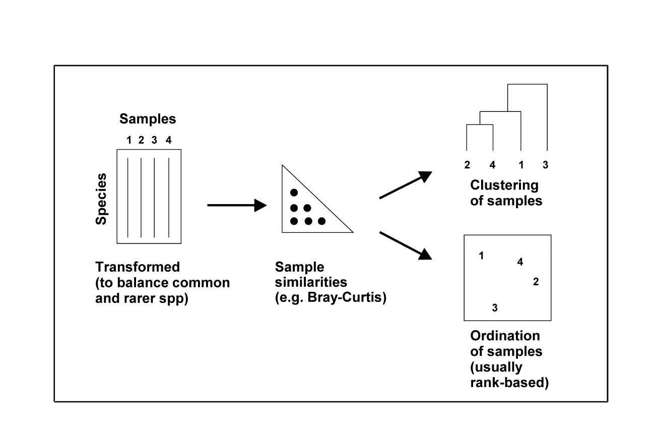
Fig. 2.1. Stages in a multivariate analysis based on (dis)similarity coefficients.
† Earlier PRIMER versions did not offer this, but v7 makes this bias correction for all coefficients that need it, e.g. for standard Euclidean distance, the pairwise-eliminated distance is multiplied by $\sqrt{p/p^\prime}$, where $p$ is the (fixed) number of variables in the matrix and $p^\prime$ the (differing) number of retained pairs for each specific distance. Manhattan uses factor $(p/p^\prime)$ but the Bray-Curtis family does not need it.
¶ The PRIMER Pre-treatment menu, under Variability Weighting, offers the choice between dividing each species through by its average replicate range, inter-quartile (IQ) range, standard deviation (SD) or pooled SD (as would be calculated in ANOVA from a common variance estimate, then square rooted). Note that this weighting uses only variability within factor levels not across the whole sample set, as in normalisation (dividing by overall SD). Clearly, variability weighting is only applicable when there are replicate samples, and these must be genuinely independent of each other, properly capturing the variability at each factor level, for the technique to be meaningful.