2.4 Species similarities
Starting with the original data matrix of abundances (or biomass, area cover etc), the similarity between any pair of species can be defined in an analogous way to that for samples, but this time involving comparison of the ith and lth row (species) across all j = 1, ..., n columns (samples).
Bray-Curtis coefficient
The Bray-Curtis similarity between species i and l is:
$$S _ {il} ^ \prime = 100 \left[ 1 - \frac{\sum_{j=1}^{n} | y_{ij} - y_{lj} | }{\sum_{j=1}^{n} ( y_{ij} + y_{lj} ) } \right] \tag{2.9}$$
The extreme values are (0, 100) as previously:
$S ^ \prime = 0 $ if two species have no samples in common (i.e. are never found at the same sites)
$S ^ \prime= 100$ if the y values for two species are the same at all sites
However, different initial treatment of the data is required, in two respects.
-
Similarities between rare species have little meaning; very often such species have single occurrences, distributed more or less arbitrarily across the sites, so that S′ is usually zero (or occasionally 100). If these values are left in the similarity matrix they will tend to confuse and disrupt the patterns in any subsequent multivariate analysis; the rarer species should thus be omitted from the data matrix before computing species similarities.
-
A different form of standardisation (species standardisation) of the data matrix is relevant and, in contrast to the samples analysis, it usually makes sense to carry this out routinely, usually in place of a transformation¶. Two species could have quite different mean levels of abundance yet be perfectly similar in the sense that their counts are in strict ratio to each other across the samples. One species might be of much larger body size, and thus tend to have smaller counts, for example; or there might be a direct host-parasite relationship between the two species. It is therefore appropriate to standardise the original data by dividing each entry by its species total over samples, and multiplying by 100:
$$y _ {ij} ^ \prime = 100 y _ {ij} / \sum_{k=1}^{n} y_{ik} \tag{2.10}$$
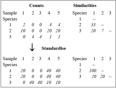
before computing the similarities ($S ^ \prime$). The effect of this can be seen from the artificial example in the following table, for three species and five samples. For the original matrix, the Bray-Curtis similarity between species 1 and 2, for example, is only $S ^ \prime = 33$% but the two species are found in strict proportion to each other across the samples so that, after row standardisation, they have a more realistic similarity of $S ^ \prime = 100$%.
Correlation coefficient
The standard product moment correlation coefficient defined in equation (2.3), and subsequently modified to a similarity, is perhaps more appropriate for defining species similarities than it was for samples, in that it automatically incorporates a type of row standardisation. In fact, this is a full normalisation (subtracting the row mean from each count and dividing by the row standard deviation) and it is less appropriate than the simple row standardisation above. One of the effects of normalisation here is to replace zeros in the matrix with largish negative values which differ from species to species – the presence/absence structure is entirely lost. The previous argument about the effect of joint absences is equally appropriate to species similarities: an inter-tidal species is no more similar to a deep-sea species because neither is found in shelf samples. A correlation coefficient will again be a function of joint absences; the Bray-Curtis coefficient will not.
Recommendation
For species similarities, a coefficient such as Bray-Curtis calculated on row-standardised and untransformed data seems most appropriate. The rarer species (often at least half of the species set) should first be removed from the matrix, to have any chance of an interpretable multivariate clustering or other analysis. There are several ways of doing this, all of them arbitrary to some degree. Field, Clarke & Warwick (1982) suggest removal of all species that never constitute more than q% of the total abundance (/biomass/cover) of any sample, where q is chosen to retain around 50 or 60 species (typically q = 1 to 3%, for benthic macrofauna samples). This is preferable to simply retaining the 50 or 60 species with the highest total abundance over all samples, since the latter strategy may result in omitting several species which are key constituents of a site which is characterised by a low total number of individuals.§ It is important to note, however, that this inevitably arbitrary process of omitting species is not necessary for the more usual between-sample similarity calculations. There the computation of the Bray-Curtis coefficient downweights the contributions of the less common species in an entirely natural and continuous fashion (the rarer the species the less it contributes, on average), and all species should be retained in those calculations.
¶ Species standardisation will remove the typically large overall abundance differences between species (which is one reason we needed transformation for a samples analysis, which dilutes this effect without removing it altogether) but it does not address the issue of large outliers for single species across samples. Transformations might help here but, in that case, they should be done before the species standardisation.
§ The PRIMER Resemblance routine will compute Bray-Curtis species similarities, though you need to have previously species- standardised the matrix (by totals) in the Pre-treatment routine. An alternative is to directly calculate Whittaker’s Index of Association on the species, see equation (7.1), since this is the same calculation except that it includes the standardisation step as part of the coefficient definition. (As Chapter 7 shows, if you are planning on using the SIMPROF test on species, described there, species standardisation is still needed). Prior to this, the Select Variables option allows reduction of the number of species, by retaining those that contribute q% or more to at least one of the samples, or by specifying the number n of ‘most important’ species to retain. The latter uses the same q% criterion but gradually increases q until only n species are left.