8.6 Example: Plymouth particle-size data
Fig. 8.15 is from Coulter Counter data of particle-size distributions for estuarine water samples from 5 sites, over 92 logarithmically increasing size-classes, based on 4 replicate samples per site (A. Bale, pers. comm.), {P}. For clarity, the line plot¶ of Fig. 8.15a shows the size distributions averaged over replicates, and some differences in profiles (multimodality etc) are apparent for the various locations, but are such differences statistically demonstrable in the context of variation among replicate water samples at a site? A Manhattan distance matrix calculated for all pairs of frequency curves from the 20 samples can be input to ordination – here metric MDS is preferred because the Shepard diagram between input distances and final distances in the MDS is perfectly linear, and has low stress (for a metric plot, especially) of 0.07, Fig. 8.15b. The plot indicates clear differences between sites and this is established by significance (at p<3%) for all pairwise ANOSIM tests, with the lowest R of 0.63 between Saltram and Devoran locations.
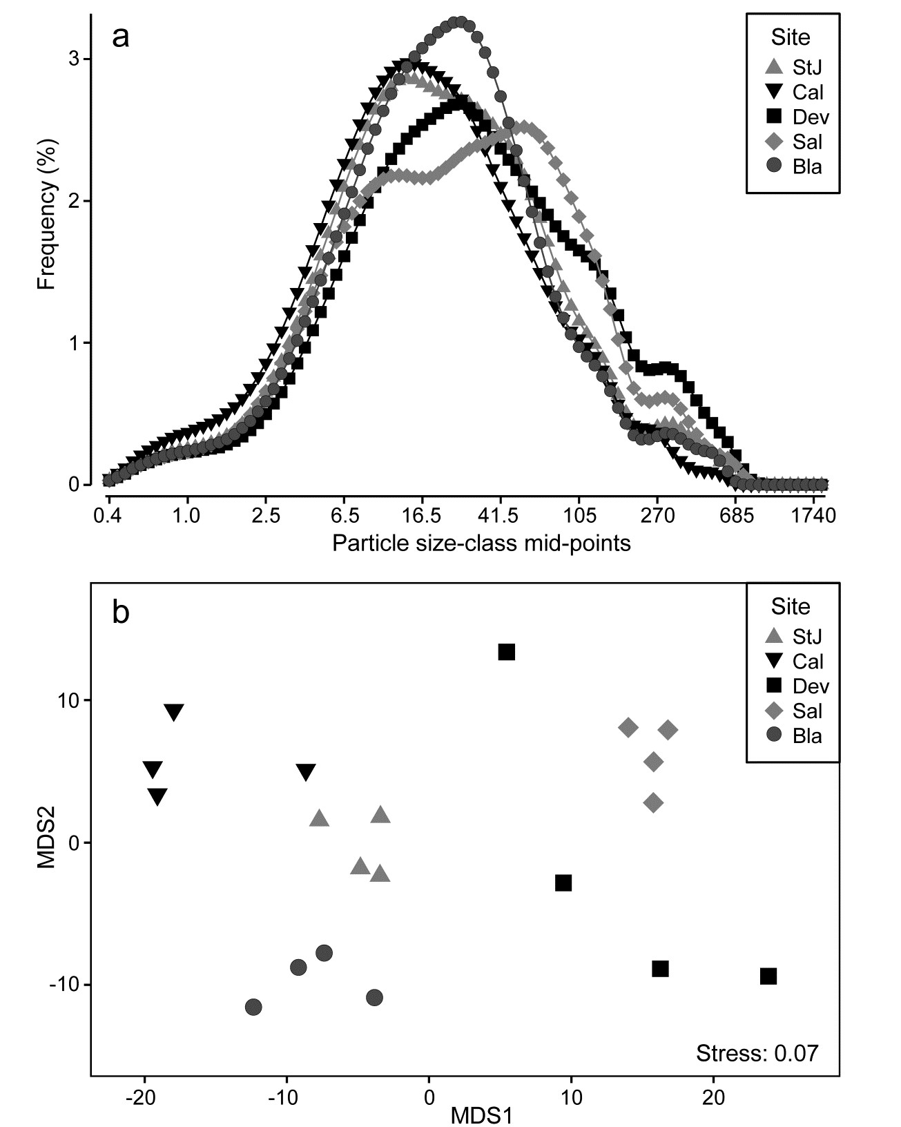
Fig. 8.15. Plymouth particle-size data {P}. a) Frequency distribution (y axis) of particle sizes in logarithmic size-classes (x axis) from water samples at 5 Plymouth sites. Frequency scale is the percentage of particulates in each of 92 classes, then averaged over 4 replicates per site. b)Metric MDS of replicate-level data based on Manhattan distances between all pairs of samples.
Ordering of the variable list
Applying multivariate methods to a matrix which is abundances not of different species, but of different size classes of a single species, has always been an (implicit) option throughout this manual, but there is one important way in which such a matrix (and the above data on particle sizes) differ from a standard community matrix: there is an explicit ordering of the variables. None of the resemblance measures (Bray-Curtis may often be appropriate again) would return different values if the ‘species’ list was re-ordered; all that matters is the degree to which the matching size-classes in the two samples have similar abundances (or relative frequencies). This was not an issue with the very smooth particle-size profiles above, but it could be when comparing (say) size-class histograms which are very ‘noisy’. That peaks for sample 1 are seen opposite troughs for sample 2 may have more to do with a choice of size interval which is too narrow, for the total frequency (arbitrarily) categorised in this way, than it does to a genuine mismatch in profiles.
A perfectly valid solution, if this is an issue, is firstly to smooth the relative frequencies (or abundances) over the size-classes before entering them to distance calculations§. Any such smoothing is ‘fair game’, provided it is done in the same way for each sample. Naturally, it increases correlation among the variables but no assumption of independence of variables is made in multivariate analysis. Quite the reverse: the techniques are designed specifically to handle and exploit correlated variables, because each sample is only treated as one ‘point’ in the analysis.
Growth curves & other repeated measures designs
Realisation that it is not necessary for the points on a curve to be independent of each other, for a method which uses the whole curve as a single (independent) replicate, naturally suggests an application to growth curves. Such a profile would be the increasing size of a specific organism (or, say, the number of hatching larvae in a single bioassay vial) monitored through time. These are (univariate) repeated measures on a single experimental/observational unit and therefore certainly not independent. But, given an appropriate design, the organisms (or the vials) are independently and randomly allocated to a specific treatment or observational condition, and statistical tests can compare this set of growth profiles with each other, among and within conditions etc, exactly as above, as a group of independent points in multivariate space. This time the variables are simply the sequence of time points, which must of course be commonly spaced across all measured profiles. In fact, this is what is known as the fully multivariate approach to univariate repeated measures designs,† except that we are here suggesting a distribution-free approach to analysis, side-stepping the need for model-based estimation of the auto-correlation structure amongst the times (‘variables’). Put simply, the problem reduces to asking whether, for example, the set of n growth profiles of organisms in group A are identifiably different in shape from the set of m profiles in B, in any respect, and consistently enough to determine significance. This needs only a measure of dissimilarity of profile pairs (e.g. Euclidean or Manhattan) and ANOSIM (/PERMANOVA).
¶ This line plot was produced in PRIMER, which has a facility for drawing line plots over the sample order in the worksheet (x axis) for each ‘species’ (y axis), with multiple species on the same plot. Of course this is the only possibility which makes sense for the usual type of community matrix, since species variables would not normally have a meaningful order to place on the x axis of a line plot (apart from the ranking by abundance of dominance plots). In this case, however, the size-class variables are automatically ordered and the natural line plot of Fig. 8.15b can be obtained by duplicating the worksheet and switching the definition of samples and variables from the Edit>Properties menu.
§ This could be by, for example, simple moving averages or more sophisticated kernel density estimation (found in many standard packages). PRIMER offers another simple form of smoothing, viz. cumulating values over the size-classes (abundances must first be sample standardised). Smoothing makes no sense for assemblage data of different species – unless the ‘nearby’ species whose abundances contribute to the moving average (say) for a specific species are defined by their taxonomic or functional affinity with that species (pooling species into higher taxa would be a crude example of this) – but is natural for ordered size-class variables
† It will not be lost on the reader that it might also be nice to have a ‘fully multivariate approach to multivariate repeated measures designs’, as arise, say, when monitoring an algal community on a marked quadrat through time. Removing a ‘quadrat effect’ in a higher-way ANOVA-type design can adjust for the fact that some quadrats have consistently different communities than others at all times, within the same ‘treatment’, but does not address the lack of symmetry in the correlation structure among times: observations at the beginning and end of a time sequence will be likely to have lower autocorrelation than adjacent times (see also the discussion in Anderson, Gorley & Clarke (2008) . A fully multivariate approach to multivariate repeated measures, using second stage analysis, is possible in limited cases, and is essentially an extension of the idea here. The ‘profile’ (in that case an entire dissimilarity matrix covering the changing community pattern over all times for a single experimental unit) becomes the single, independent point in a multivariate space which, along with other (matrix) points, we can enter into ANOSIM tests, MDS etc. Chapter 16 gives an example of such a rocky-shore experiment to monitor algal recolonisation of quadrats under different clearance conditions