5.3 Diagnostics: Adequacy of MDS representation
-
Is the stress value small? By definition, stress reduces with increasing dimensionality of the ordination; it is always easier to satisfy the full set of rank order relationships among samples if there is more space to display them. The scree plot of best stress values in 2, 3, 4,.. dimensions therefore always declines. Conventional wisdom is to look for a ‘shoulder’ in this plot, indicating a sudden improvement once the ‘correct’ dimensionality is found, but this rarely happens. It is also to miss the point about MDS plots: they are always approximations to the true sample relationships expressed in the resemblance matrix. So for testing and many other purposes in this manual’s approach we will use the full resemblance matrix. The 2-d and 3-d MDS ordinations are potentially useful to give an idea of the main features of the high dimensional structure, so the valid question is whether they are a usable approximation or likely to be misleading.
One answer to this is through empirical evidence and simulation studies of stress values. Stress increases not only with reducing dimensionality but also with increasing quantity of data, but a rough rule-of-thumb, using the stress formula (5.1), is as follows.†
Stress <0.05 gives an excellent representation with no prospect of misinterpretation (a perfect representation would probably be one with stress <0.01 since numerical iteration procedures often terminate when stress reduces below this value§).
Stress <0.1 corresponds to a good ordination with no real prospect of a misleading interpretation; higher-dimensional solutions will probably not add any additional information about the overall structure (though the fine structure of any compact groups may bear closer examination).
Stress <0.2 still gives a potentially useful 2-dimensional picture, though for values at the upper end of this range little reliance should be placed on the detail of the plot. A cross-check of any conclusions should be made against those from an alternative method (e.g. the superimposition of cluster groups suggested in point 5 below), higher-dimensional solutions examined or ways founds of reducing the number of samples whose inter-relationships are being represented, by averaging over replicates, times, sites etc or by selection of subsets of samples to examine separately, in turn.
Stress >0.3 indicates that the points are close to being arbitrarily placed in the ordination space. In fact, the totally random positions used as a starting configuration for the iteration usually give a stress around 0.35–0.45. Values of stress in the range 0.2–0.3 should therefore be treated with a great deal of scepticism and certainly discarded in the upper half of this range. Other techniques will be certain to highlight inconsistencies.
-
Does the Shepard diagram appear satisfactory? The stress value totals the scatter around the regression line in a Shepard diagram, for example the low stress of 0.05 for Fig. 5.1 is reflected in the low scatter in Fig. 5.2. Outlying points in the plot could be identified with the samples involved; often there are a range of outliers all involving dissimilarities with a particular sample and this can indicate a point which really needs a higher-dimensional representation for accurate placement, or simply corresponds to a major error in the data matrix.
-
Is there distortion when similar samples are connected in the ordination plot? One simple check on the success of the ordination in dissimilarity-preservation is to specify an arbitrary similarity threshold (in practice try a series of thresholds) and join all samples in the ordination whose similarity is greater than this threshold. This is shown for the Exe data in Fig. 5.3a, at a similarity level of 30% and indicates no strong inconsistencies of the MDS distances with the similarity matrix (e.g. the group 5,10 is further from 6,11 than the latter is from 7,8,9, and clearly of greater dissimilarity). However, though low, the stress is not zero, and it is clear that some of this comes from representation of the detailed structure of the (looser) 12-19 group. For example, Fig. 5.3a shows that sample 15 is more similar to 16 than it is to either 18 or 17, which is not the picture seen from the 2-d MDS.
-
Is the ‘minimum spanning tree’ consistent with the ordination picture? A similar idea to the above is to construct the minimum spanning tree (MST, Gower & Ross (1969) ). All samples are connected on the MDS plot by a single line which is allowed to branch but does not form a closed loop, such that the sum along this line of the relevant pairwise dissimilarities is minimised (again, this is taken from the original dissimilarity matrix not the distance matrix from the ordination points, note). Inadequacy is again indicated by connections which look unnatural in the context of placement of samples in the MDS configuration. The MST is shown for the Exe data in Fig. 5.3b and the same point about stress in the 2-d MDS for samples 15-18 can be seen. Similarly, there is clearly higher-dimensional structure than can be seen here among samples 12-14 and their relation with 19, since the MST shows that 12 is more similar to 13 than it is to the apparently intermediate point 14, and the MST does not take the apparently shortest route to sample 19. A lower stress must be obtained for a 3-d MDS (it drops a little to 0.03 here), and Fig. 5.3c of the 3-d MDS does show, for example, that points 12,13 are close and 14 a little separated, as Figs. 5.3a, 5.3b and the cluster analysis Fig. 5.4 would all suggest. (Viewing 3-d pictures in 2-d is not always easy but can be very much clearer with dynamic rotation of the 3-d plot, which is allowed in PRIMER as with many other plotting programs). When 2-d stress is as low, as it is here, the extra difficulty of displaying a 3-d solution for such a marginal improvement must be of doubtful utility, but in many cases there will be real interpretational gains in moving to a 3-d MDS solution.
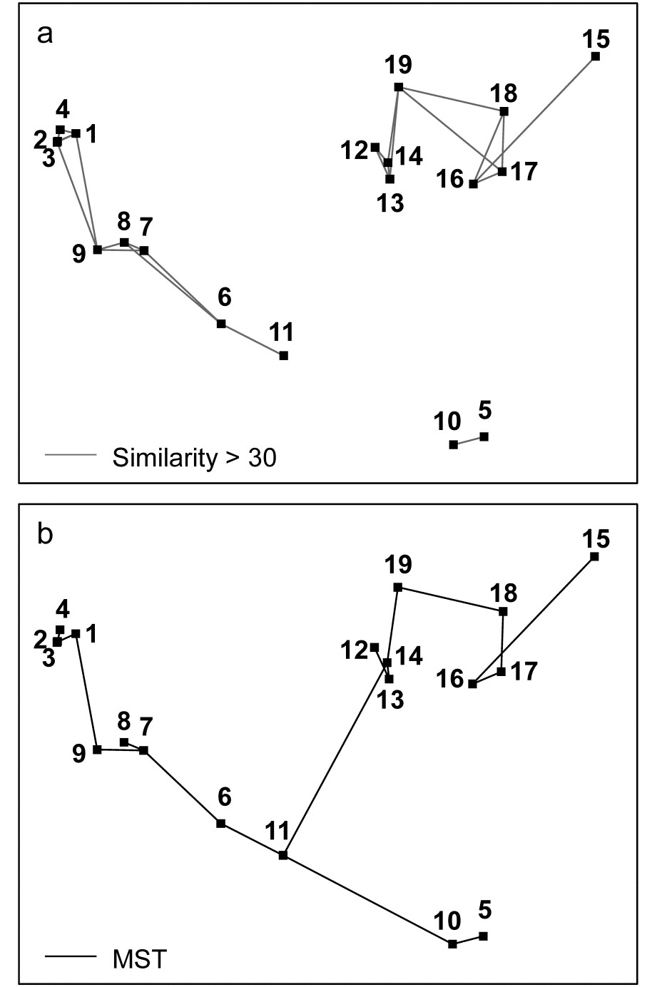
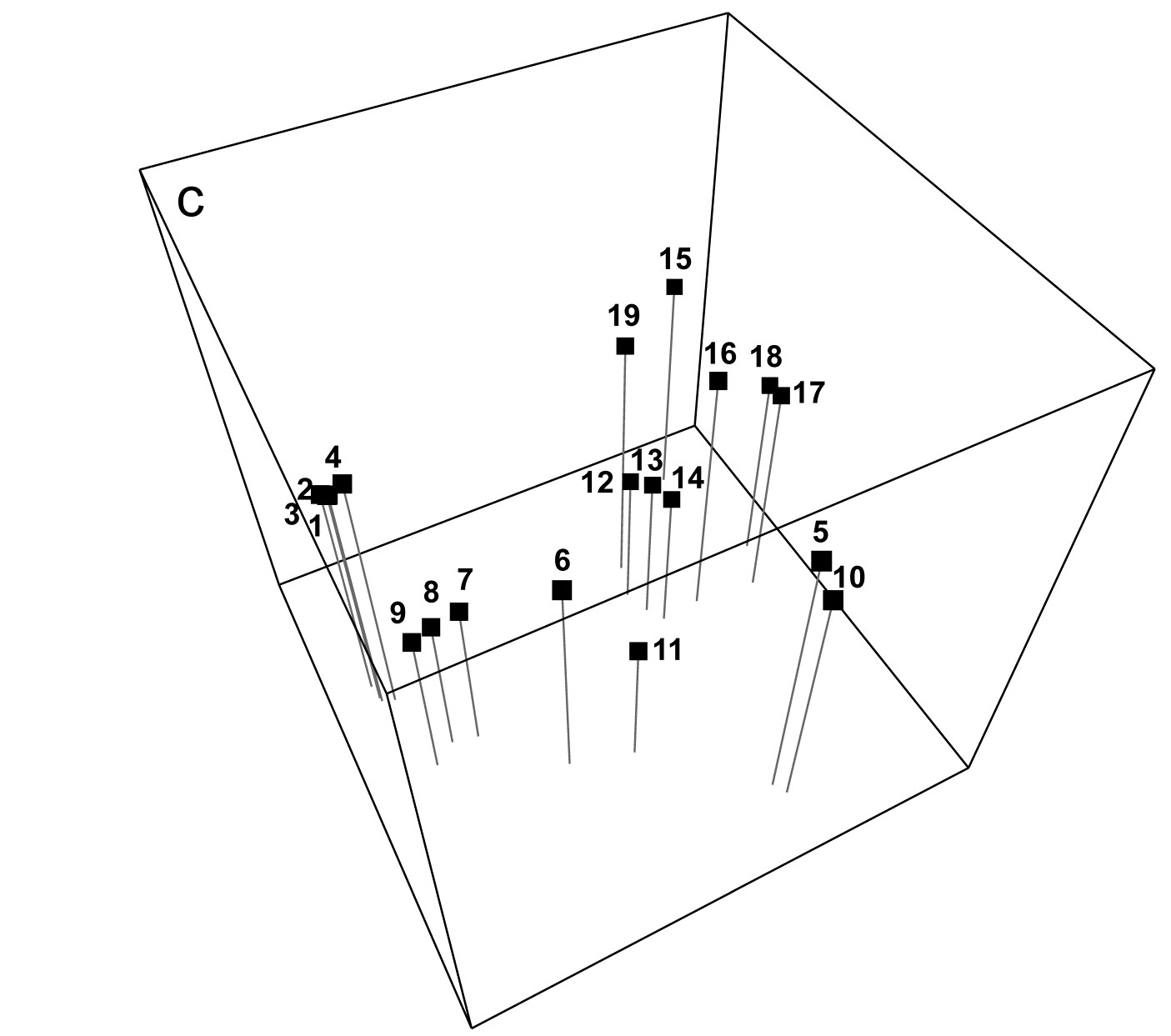
Fig. 5.3. Exe estuary nematodes {X}. a) & b) Two-dimensional MDS configuration, as in Fig. 5.1 (stress = 0.05), with:
a) samples >30% similar (by Bray-Curtis) joined by grey lines;
b) the minimum spanning tree through the dissimilarity matrix indicated by the continuous line.
c) Three-dimensional MDS configuration (stress = 0.03).

Fig. 5.4. Exe estuary nematodes {X}. Dendrogram of the 19 sites, using group-average clustering from Bray-Curtis similarities on $\sqrt{}\sqrt{}$-transformed abundances. The four site groups (1 to 4) identified by Field et al (1982) at a 17.5% similarity threshold are indicated by a dashed line (they also split the two tightly clustered sub-groups in group 1). A 35% slice is also shown.
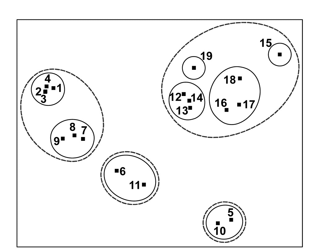
Fig. 5.5. Exe estuary nematodes {X}. Two-dimensional MDS configuration, as in Fig. 5.1 (stress = 0.05), with clusters identified from Fig. 5.4 at similarity levels of 35% (continuous line) and 17.5% (dashed line).
- Do superimposed groups from a cluster analysis distort the ordination plot? The combination of clustering and ordination analyses can also be an effective way of checking the adequacy and mutual consistency of both representations. Slicing the dendrogram of Fig. 5.4 at two (or more) arbitrary similarity levels determines groupings which can be identified on the 2-d ordination by a closed region around the points. (PRIMER uses its own ‘nail and string’ algorithm to produce smoothed convex hulls of the points in each cluster, where the degree of smoothing is under user control, with a smoothing parameter of zero resulting in the convex hull). Here the approximately 17.5% similarity used by the original Field, Clarke & Warwick (1982) paper is shown by the dashed line in Figs. 5.4 and 5.5, and a continuous line shows the clusters produced from slicing the dendrogram between about 30-45% similarity. It is clear that the agreement between the MDS and the cluster analysis is excellent: the clusters are well defined and would be determined in much the same way if one were to select clusters by eye from the 2-dimensional ordination alone. One is not always as fortunate as this, and a more revealing example of the benefits of viewing clustering and ordination in combination is provided by the data of Fig. 4.2.¶
† There are alternative definitions of stress, for example the stress formula 2 option provided in the MDSCAL and KYST programs. This differs only in the denominator scaling term in (5.1) but is believed to increase the risk of finding local minima and to be more appropriate for other forms of multivariate scaling, e.g. multidimensional unfolding, which are outside the scope of this manual.
§ This is under user control with the PRIMER routine, for example, but the default is 0.01.
¶ One option within PRIMER is to run CLUSTER on the ranks of the similarities rather than the similarities themselves. Whilst not of any real merit in itself (and not the default option), Clarke (1993) argues that this could have marginal benefit when performing a group-average cluster analysis solely to see how well the clusters agree with the MDS plot: the argument is that the information utilised by both techniques is then made even more comparable.