16.3 Example: Amoco-Cadiz oil spill

Applying this (BVStep) procedure to the 125-species set from the Bay of Morlaix, a smallest subset of only 9 species can be found, whose similarity matrix across the 21 samples correlates with that for the full species set, at $\rho \ge 0.95$. The MDS plot for the 21 samples based only on these 9 species is shown in Fig.16.3b and is seen to be largely indistinguishable from 16.3a. The make-up of this influential species set is discussed later but it is important to realise, as often with stepwise procedures, that this may be far from a unique solution. There are likely to be other sets of species, a little larger in number or giving a slightly lower $\rho$ value, that would do a (nearly) equally good job of ‘explaining’ the full pattern.

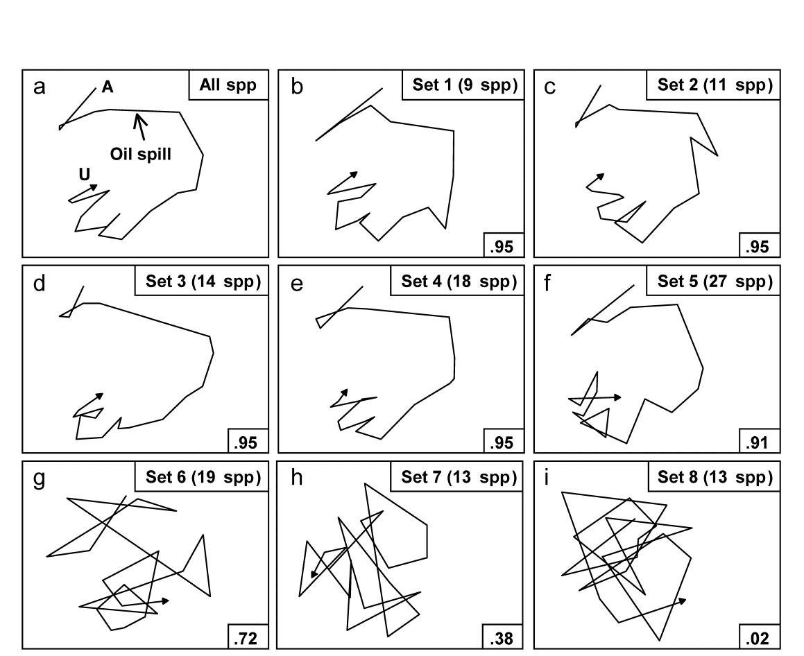
Fig. 16.3. Amoco-Cadiz oil spill {A}. MDS plots from 21 samples (approximately quarterly) of macrobenthos in the Bay of Morlaix (Bray-Curtis on 4th-root transformed abundances). a) As Fig. 16.1 but discarding the rare species, leaving 125; b)–f) based on a succession of five, small, mutually exclusive subsets of species, generated by the BEST/BVStep option, showing the high level of matching with the full data ($\rho$ values in bottom right of plots, and number of species in top right); g)–i) after successive removal of the species in previous plots, the ability to match the original pattern by selecting from the remaining species rapidly degrades (stress = 0.09, 0.08, 0.08, 0.08, 0.12, 0.12, 0.21, 0.24, 0.24 respectively).
 

One interesting way of seeing this is to discard the initial selection of 9 species, and search again for a further subset that produces a near-perfect match ($\rho \ge 0.95$) to the pattern for the full set of 125 species. Fig. 16.3c shows that a second such set can be found, this time of 11 species. If the two sets are discarded, a third (of 14 species), then a fourth (of 18 species) can also be identified, and Fig. 16.3d and e again show the high level of concordance with the full set, Fig. 16.3a. There are now 73 species left and a fifth set can just about be pulled out of them (Fig. 16.3f), though now the algorithm terminates at a genuine maximum of $\rho$; a match better than $\rho = 0.91$ cannot be found by the stepwise procedure, even after several attempts with different random starting positions. If these (27) species are also discarded, the ability of the remaining 46 species to reconstruct the initial pattern degrades slowly (Fig. 16.3g) then rapidly (Fig. 16.3h and i), i.e. little of the original ‘signal’ remains.

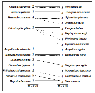
Clarke & Warwick (1998a) discuss the implication of these plots for concepts of structural redundancy in assemblages (and, arguably, for functional redundancy, or at least compensation capacity). They investigate whether the various sets of species ‘peeled’ out from the matrix have a similar taxonomic structure. For example, Table 16.2 displays the first and second ‘peeled’ species lists and defines a taxonomic mapping coefficient, used to measure the degree to which the first set has taxonomically closely-related counterparts in the second set, and vice-versa. (Note that taxonomic relatedness concepts are the basis of several indices used in Chapter 17, this specific coefficient being the $\Theta ^ +$ of eqn. 17.8) A permutation test can be constructed that leads to the conclusion that the peeled subsets are more taxonomically similar (i.e. have greater taxonomic coherence) than would be expected by chance. The number of such coherent subsets which can be ‘peeled out’ from the matrix is clearly some measure of redundancy of information content.

Table 16.2. Amoco-Cadiz oil spill {A}. Illustration of taxonomic mapping of the second and third ‘peeled’ species subsets (i.e. those underlying Fig. 16.3c,d), from the successive application of BVStep, highlighting the (closer than random) taxonomic parallels between the species sets which are capable of ‘explaining’ the full pattern of Fig. 16.3a. Continuous lines represent the closest relatives in the right-hand set to each species in the left-hand set (underlined values are the number of steps distant through the taxonomic tree, see Chapter 17 for examples). Dashed lines map the right-hand set to the left-hand (non-underlined values are again the taxonomic distances). The taxonomic mapping similarity coefficient, M, averages the two displayed mean taxonomic distances (denoted $\Theta ^ + $ in Chapter 17).

 

Viewed at a pragmatic level, the message of Fig. 16.3 is therefore clear. It is not a single, small set of species which is responsible for generating the observed sample patterns of Fig. 16.1, of disturbance and (partial) recovery superimposed on a seasonal cycle. Instead, the same temporal patterns are imprinted several times in the full species matrix. The steady increase in size of successive ‘peeled’ sets reflects the different signal-to-noise ratios for different species, or groups of species. The signal can be reproduced by only a few species initially but, as these are sequentially removed, the remaining species have increasingly higher ‘noise’ levels, requiring an ever greater number of them to generate the same strength of ‘signal’. Clarke & Warwick (1998a) give further macrobenthic examples, of time series from Northumberland subtidal sites, whose structural redundancy is at a similar level (4–5 peeled subsets), though this is by no means a universal phenomenon (M G Chapman, pers. comm., for rocky shore assemblages; Clarke & Gorley (2006 or 2015) , for zooplankton communities, both of which examples are much less species-rich in the first place).