6.16 Example: NZ kelp holdfast macrofauna
We now consider the fully nested design, C(B(A)). In north-eastern New Zealand, Anderson, Diebel, Blom et al. (2005) examined assemblages of invertebrates colonising kelp holdfasts at three spatial scales: 4 locations (A), with 2 sites (B) per location, sampling 2 areas (C) at each site and with 5 replicate holdfasts per area, {n}. This data is covered in detail in the PERMANOVA+ manual, Anderson, Gorley & Clarke (2008) ¶. Since B and C have only 2 levels, there can be no concept of them being ‘ordered’ or not; A is also seen as unordered. The test statistics are therefore $R$ and $\overline{R}$, case 3d in Table 6.4, giving for A: $R = 0.81$, B: $\overline{R}= 0.38$ and C: $\overline{R}= 0.26$.
These three ANOSIM R statistics are again directly comparable with each other. Their increase in size as the spatial scale increases is coincidental; they do not reflect accumulation of differences at all the spatial scales but only the additional assemblage differences when moving from replicates (with spacing at metres) to areas (at 10’s of metres) to sites (100’s of metres to kms) to locations (100’s of km). Thus, they can be seen as non-parametric equivalents of the univariate variance components (or the multivariate components of variation in PERMANOVA): the area differences
are small ($\overline{R} = 0.26$) in relation to assemblage variability from one holdfast to another, somewhat larger between sites (0.38), in relation to changes between areas, and very large among locations (0.81), relative to change in sites within those locations. This is in stark contrast to the conclusions one might draw from looking only at the significance levels (as seen from the permutation distributions under the null hypotheses, Fig. 6.16), A: p=1%, B: p=1.2%, C: p<<0.01%, a result of the very different numbers of replicates, and thus possible permutations (105, 85 and 1268). As always, it is the $R$ values which give the effect sizes.
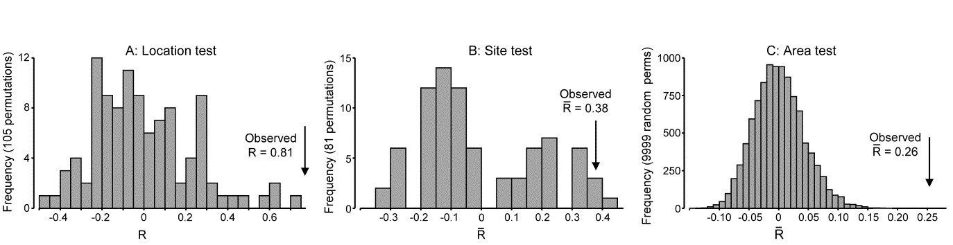
Fig. 6.16. NZ kelp holdfast fauna {n}. Null distributions by permutation for 3-factor fully nested (unordered) ANOSIM tests, C(B(A)), with 5 replicates from each of 2 areas (C), nested in 2 sites (B), nested in 4 locations (A). Very large numbers of permutations possible for the lowest level test of areas, so 9999 selected at random; all permutations are computed for site test (81) and location test (105).
Pairwise tests are only meaningful at the top level of such a nested design and there are insufficient permutations here (3) to make these at all informative. The best way, as always, to follow up the global ANOSIM tests, and visualise the effect sizes, is an MDS based on averaged data (but see footnotes on pages 5.9 & 6.15). Here Fig. 6.17 averages the (square root-transformed) replicate counts for the 16 areas, recomputes Bray-Curtis and the nMDS plot re-affirms the test results.
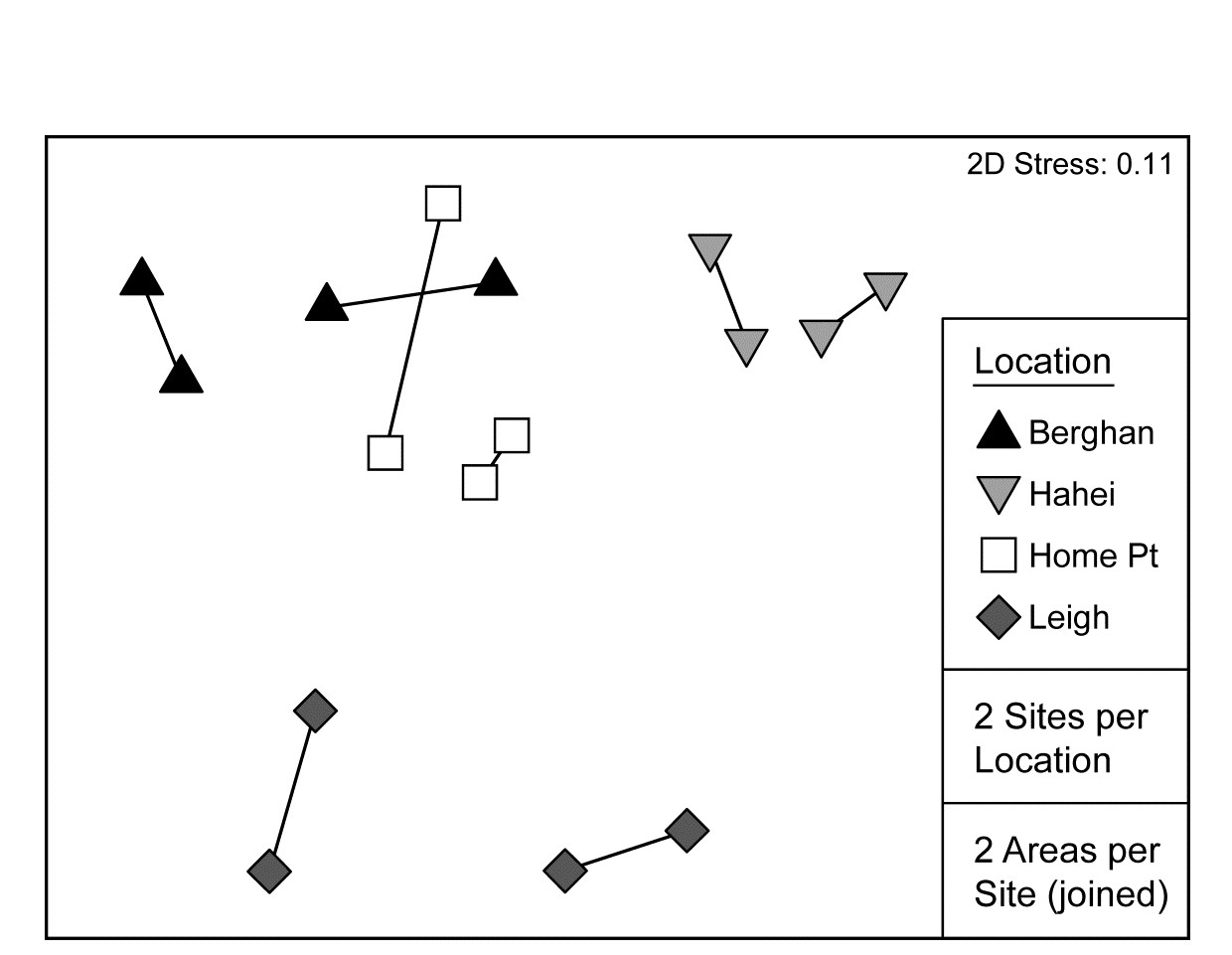
Fig. 6.17. NZ kelp holdfast fauna {n}. nMDS (on Bray-Curtis) of square-rooted abundances of 351 species, averaged over five replicates holdfasts in each area (nested in site and location).
There is a minor technical issue, in the sequence of nested ANOSIM tests, as to how best to combine the original replicates to provide ‘area replicates’ for a test of site, and then how best to combine the areas to provide ‘site replicates’ for a test of locations. There are many possibilities: PERMANOVA uses centroids calculated in the high-dimensional resemblance space (see Anderson, Gorley & Clarke (2008) ) whereas the rank-based approach in PRIMER was given on page 6.6 for the two-way nested case (the original resemblances are ranked, then averaged and re-ranked, at each level). Averaging the similarities rather than their ranks is another possibility, as is averaging the data, both transformed (as in Fig. 6.17) or untransformed. Only slight variations would be likely from the different choices, though experience suggests that averaging untransformed data makes the greatest difference. But in one situation even this might be considered appropriate, namely when the original replicates are sufficiently sparse and unreliable not to constitute a fair reflection of the assemblage structure at all: to pool them (i.e. average untransformed counts) and run the 3-way nested case as 2-way nested for A and B(A) tests (2g-n, Table 6.3) might then be preferable.
¶ We are ignoring for the purposes of this illustration that, as Anderson, Gorley & Clarke (2008) explain, the holdfasts will have different volumes and, even after we have attempted to correct for this by standardising all samples to relative composition not absolute numbers, there may still be some artefactual dissimilarity arising from higher species richness in larger holdfasts. PERMANOVA tests can attempt to model the ‘nuisance’ effects of covariates such as this, through a linear regression, and thereby adjust the C(B(A)) tests (as Anderson, Gorley & Clarke (2008) do in this case); clearly nothing similar could ever be available in the non model-based approach here. However, such biases from unequal sample sizes will still remain in any ordination configuration, whatever the approach, and it should be examined by bubble plots of (here) holdfast volume on the area MDS. Characteristic indicators of a problem are that all the outlying points have low sample volumes (which does not happen here). Presence/absence analyses will be most prone to this artefact, so where such a problem is expected, some amelioration is likely from using less severe transforms – here the mild square root is used – or possibly dispersion weighting (Chapter 9). This downweights the contribution of highly abundant, but highly variable, species without also effectively ‘squashing’ species with low counts (but consistent over replicates) to presence/absence, as severe transformations will do.