18.4 Example: Loch Creran macrobenthos
Gage & Coghill (1977) collected a set of 256 soft-sediment macrobenthic samples along a transect in Loch Creran, Scotland {c}, data which have little or no evidence of a trend or spatial group structure and will therefore be useful here in illustrating a potential bootstrapping artefact, discussion of which we postponed from the previous page. For this example, 16 cores are pooled at a time, giving 16 replicates spaced along the transect, each having sufficient biological material to fairly reflect the community (an average of 26 species per replicate). A 2-level group factor is defined as the first and second halves of the transect (1-8 for group A and 9-16 for group B) and Fig. 18.4a shows the resulting mMDS plot. A stress of 0.27 on only 16 points is too high for a reliable plot, even for a metric MDS, and the Shepard plot of 18.4b shows the inadequacy of metric linear regression (through the origin) for this 2-d ordination. Nonetheless, whilst there is some suggestion that the ‘centres’ for the two groups are not in precisely the same position (with 5 of the 8 replicates from group A being to the left and bottom of those for group B), it is no surprise to find that an ANOSIM test (or a PERMANOVA test), on the Bray-Curtis similarities from the untransformed species counts in the 67-d samples $\times$ species matrix, does not distinguish the two groups at all. But what happens to the bootstrap averages?
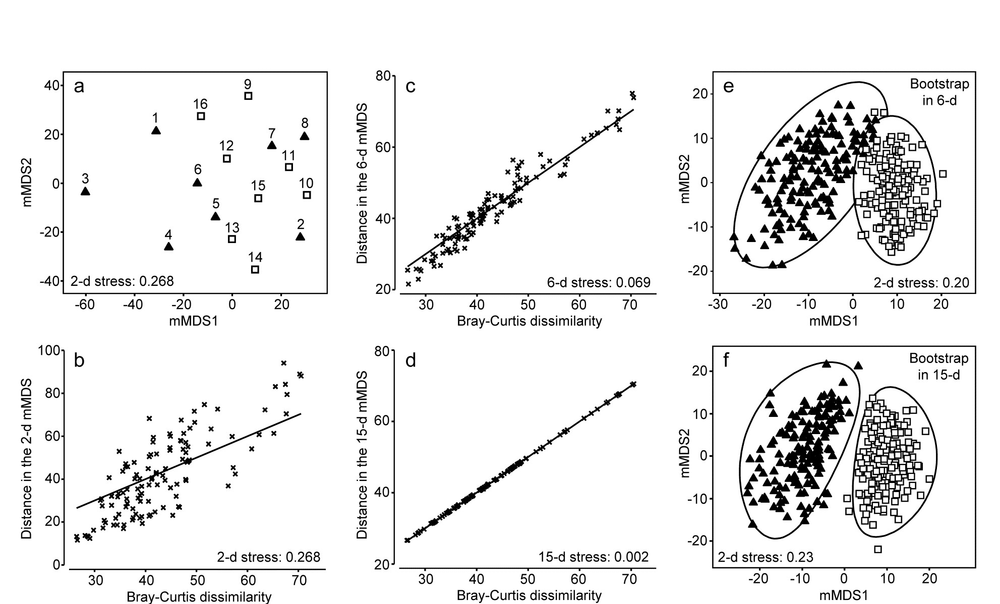
Fig. 18.4. Loch Creran macrobenthos {c}. (a) mMDS plot of (pooled) samples, 1-16, along a single transect, from untransformed data and Bray-Curtis dissimilarities. Triangles and squares denote groups A (1-8) and B (9-16). b-d) Shepard diagrams for the mMDS plots of these 16 samples in 2-d, 6-d and 15-d. e) Bootstrap average regions (95%) for groups A and B, symbols as in (a), by bootstrapping co-ordinates of the 16 samples in the 6-d mMDS approximation to the original 67-d space (Pearson matrix correlation $\rho = 0.968$, of those inter-point distances with the original resemblance matrix). f) Regions as in (e) but by bootstrapping co-ordinates in the 15-d mMDS space, which in this case perfectly preserves the Bray-Curtis similarities from the full space, as shown by (d), and $\rho = 1$.
Artefact of bootstrapping in high dimensions
The 95% region estimates for the means of the two groups, whilst they will inevitably be ‘centred’ in different places, would be expected to overlap, but this is not what happens when bootstrap averages are calculated separately for the two sets of 8 replicates in their full (67-d) species space and then ordinated into lower dimensions, as shown in the 2-d mMDS of Fig. 18.5.
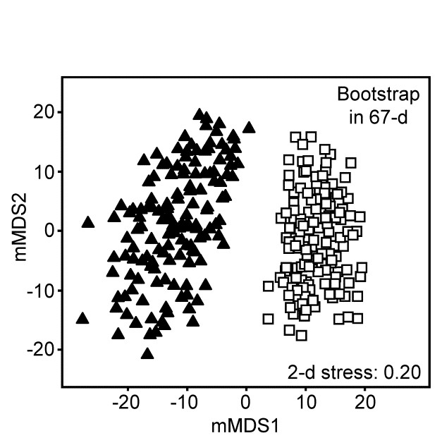
Fig. 18.5.Loch Creran macrobenthos {c}. 2-d mMDS of bootstrap averages in the original 67-d species space, for groups A and B.
What has gone horribly wrong here? The answer lies in the vastness of high-dimensional space¶. Bootstrap samples ‘work’, in the sense of giving a plausible set of alternative samples (with the same properties) to the set we actually did obtain, because the spread of values produced, along a line, in a plane, in a 3-d box etc, cover much the same interval, areal and spatial extents as the original samples. However, this feature gradually starts to disappear for increasingly higher dimensions. This data set contains only 16 points, but these are in 67-dimensional space. Many of the points could ‘have some dimensions to themselves’, purely by chance, when there are no real differences in the two communities, e.g. because of the sparse presence of many species in a typical assemblage matrix. The two groups of samples will thus occupy a somewhat different set of dimensions (many dimensions will be found in both sets, of course, but some will only be found in one or other group). On repeated sampling separately from each of the groups, it is inevitable that bootstrap averages for a group will remain in its own subset of dimensions. Those averages vary over a tighter range than the original samples – that is the nature of averages – and the non-identity of the two sets of dimensions will cause the bootstrap averages to shrink apart so that, even in a low-d ordination, the two groups will not overlap. This oversimplifies a complex situation but is likely to be one of the basic reasons why the high-d bootstrap artefact is seen.
This way of posing the problem immediately suggests a possible solution, namely to bootstrap the samples in a much lower-d space, which nonetheless retains essentially all the information present in the original resemblances from the 67-d samples $\times$ species matrix. Here, we have only 16 samples and a 15-d mMDS can, in this case, near-perfectly† reconstruct the set of among-sample Bray-Curtis resemblances in 15-d, as can be seen in the Shepard diagram of Fig. 18.4d. However, the 15-d mMDS of Fig. 18.4f shows that the high-d artefact is still present, though apparently substantially reduced. This is perhaps unsurprising, given there are still as many dimensions as points, and we need to search for a lower-dimensional space in which to create the bootstrap averages.
The technique we have used in previous chapters to measure information loss in replacing a resemblance matrix with an alternative is simple matrix correlation of the two sets of resemblances. Here, in the context of metric MDS, which tries to preserve dissimilarity values themselves, it would be appropriate to use a standard (Pearson) correlation $\rho$, rather than the non-parametric Spearman correlation which fits better to preserving rank orders of resemblances in nMDS. A suggested procedure is therefore to ordinate the data by mMDS, from the chosen dissimilarity matrix, into increasingly higher dimensions, until a predetermined threshold for $\rho$ is crossed (say $\rho > 0.95$ or $\rho > 0.99$). The $\rho$ value is almost sure to increase monotonically with the dimension, $m$. The process can probably start with $m \ge 4$, since evidence suggests the high-d artefact does not trouble such relatively low-d space. At the upper end, as $m$ gets much larger than 10, the artefact can become non-negligible, especially if (as for the current example) this is nearing the total sample size in the original data. This suggests that the search is made over $4 \le m \le 10$ (and this will certainly produce $\rho$ values in the range 0.95-0.99).
In the current Loch Creran example, an mMDS in $m = 6$ dimensions provides a reasonable linear fit to the original resemblance values, as shown in Fig. 18.4c (for which $\rho = 0.97$). The co-ordinates of the sample points in this m-dimensional mMDS space are now used to produce a large number of bootstrap averages (b) for each group. b ≥ 100 is recommended, though lower values may have to be used if there are many groups, in order to obtain mMDS region plots in a viable computation time. Here, for only two groups, b = 150 averages were taken from each. Euclidean distances are then computed among these bootstrap averages, this being the relevant resemblance matrix for points in ordination space, naturally§. These are then input to metric MDS to obtain the final 2- or 3-d ordination plot and the smoothed region estimates, as previously described for the S Tikus data of Fig. 18.2 and 18.3 (this is the procedure that was followed for those earlier plots, selecting m=7, for which $\rho$ >0.95). The 95% region plot for the Creran data (Fig. 18.4e) now shows the two groups overlapping, as expected‡.
A somewhat subtle but important consequence of this solution to the high-d bootstrap artefact is that it also addresses the issue raised in the footnote on page 18.2, that simple averages of replicates in species space will often not occupy the centre of gravity of those replicates when they and the averages are ordinated together, using a similarity such as Bray-Curtis (or any biological measure responding to the presence/ absence structure in the data). But now the averaging is carried out in the Euclidean distance-based mMDS space which approximates those similarities so, for each group, the mean of the bootstrap averages is just their centre of gravity (in the m-dimensional space).⸙ And theoretical unbiasedness of the bootstrap method (a univariate result which carries over to multivariate Euclidean space) dictates that this mean will be close to the group average of the original replicates, when the latter is calculated in the m-dimensional space. (This is not, of course, the same as computing these averages in the original species space and ordinating them, along with the replicates, into m dimensions.)
Thus, in Fig. 18.2c for example, the means shown should be close to the centres of gravity of the clouds of bootstrap averages in 18.2b; they can only not be so because of the distortion involved in the final step of approximating the m-dimensional space by a 2-d mMDS solution. Thus the means are usually worth displaying, as a further guide to such distortion.
A final example of bootstrapping is one with slightly different numbers of replicate samples across groups, though bootstrap averages are calculated in just the same way and without bias from the varying sampling effort for one of the means (again see footnote ⸙).
¶ “Space is big. Really big. You just won't believe how vastly, hugely, mindbogglingly big it is. I mean, you may think it's a long way down the road to the chemist's, but that's just peanuts to space.” Douglas Adams, 1978, The Hitchhiker’s Guide to the Galaxy. Not a quote about high-d space, but it could have been!
† Euclidean distances among k points can always be represented in k-1 dimensions but here we are dealing with biological resemblance measures which are never ‘metrics’, so this can only be achieved in general with a mix of real and imaginary axes (i.e. in complex space, see for example Fig. 3.4 of Anderson, Gorley & Clarke (2008) ). A real-space mMDS can nearly always get close to recreating the original dissimilarities however; often near-perfectly, as here.
§ Do not confuse this with making Euclidean distance assumptions for the original samples $\times$ species matrix! We are still computing, say, Bray-Curtis dissimilarities among the samples, exactly as previously, but then we approximate those by Euclidean distances among points in m dimensions (this is what the Shepard diagram shows and is what ordination is all about). For each of g groups, a bootstrap average is then a simple centroid (‘centre of gravity’) of n bootstrap samples drawn with replacement from that group’s n points in this Euclidean space. b such averages are produced for each group, and it is the (Euclidean) distances among those b$\times$g points which are input to the final mMDS, to obtain plots such as Fig. 18.4e.
‡ It is a mistake to expect an exact parallel between overlap of bootstrap regions and the significance of (say) pairwise ANOSIM tests, in the way that (with careful choice of confidence probabilities) univariate confidence intervals, based on normality, can be turned into hypothesis tests. Bootstraps do not give formal confidence regions and a number of approximations are made (e.g. sample size is often small for bootstrapping, the final display is in approximate low-d space, etc); in contrast ANOSIM is an exact permutation test, but utilises only the ranks from the full resemblance matrix. Nonetheless, as we saw for S Tikus corals, the relative positioning and size of regions in these plots can add real interpretative value, following hypothesis testing.
⸙ And this also sidesteps the issues raised in the last paragraph of the footnote on page 18.2. Averaging over unbalanced numbers of replicates for the differing groups will not now introduce a bias coming from the relative species richness of these averages, since that averaging is in the Euclidean space of the low-d mMDS, not the species matrix. Thus it can be carried out with impunity on heavily transformed (or even presence/absence) samples from unbalanced group sizes. However, the same remarks apply now, about breaking the link to the species, as to the centroids in PCO space calculated in PERMANOVA+ ( Anderson, Gorley & Clarke (2008) ), to which these mMDS spaces have a strong affinity. The differences are that the PERMANOVA+ centroids are calculated in the full PCO space (and in general will have real and imaginary components) whilst the mMDS is an approximation in real space; also that lower-d plots are produced by projection through the higher axes with PCO but by placement of points in low-d in mMDS (in such a way as to optimise the fit to the actual resemblances).