7.9 Example: Tasmanian meiofauna
Another clear generalisation is to a 2-way rather than 1-way layout, illustrated by the 16 meiofaunal cores from Eaglehawk Neck, Tasmania, Fig. 6.7. The MDS for the 59 nematode and copepod species from two crossed factors, treatments (disturbed or undisturbed sediment from activity of soldier crabs) and blocks (locations B1 to B4 across the sandflat) is again seen in Fig. 7.12, this time with the 16 pairs of dissimilarities between treatments for the same block shown by dashed lines. Clearly, they are the only dissimilarities appropriate to a SIMPER analysis of which species are primarily responsible for the community change between Disturbed and Undisturbed conditions which was established in Chapter 6 by the 2-way ANOSIM test, and they are the similarities used in the species breakdown produced by the 2-way crossed SIMPER calculations (e.g. Platell, Potter & Clarke (1998) ).
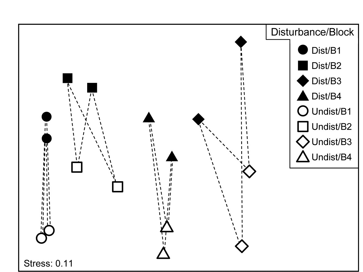
Fig. 7.12. Tasmania, Eaglehawk Neck {T}. nMDS of 2 replicates from each of 4 blocks under disturbed/undisturbed conditions (see Fig. 6.7). 2-way SIMPER for the species contributing to the disturbance effect uses only the dissimilarities indicated by dashed lines, i.e. between disturbance conditions within each block.
A 1-way SIMPER on the treatment factor in this case would look at all 64 dissimilarities between the 8 samples in each of the two conditions, but this mixes up effects which are due to treatment with those due to block differences, since for example they would use the dissimilarity between a Disturbed sample in Block 1 and an Undisturbed sample in Block 2. A separate 1-way SIMPER analysis could be run on the treatment difference for each of the blocks, but the 2-way SIMPER here combines these neatly into a more succinct table, and there seems little evidence (from the MDS plot) of the disturbance effect differing to any great extent from block to block – this appears to be an approximately additive 2-factor pattern.
Other techniques for identifying species
A significant weakness of the SIMPER approach is its limitation to comparing two identified groups of samples at a time, sometimes leading to very large numbers of tables which are difficult to synthesise. In some contexts, a grouping structure of samples is not even observed or expected, the sample pattern being that of a continuous gradient (or gradients). What is needed here is a more holistic technique, identifying the set of influential species which between them are able to capture the full multivariate pattern (whether clustered or a gradation), and which operates with any appropriately-defined similarity coefficient. A solution to this is presented later, in Chapter 16 on comparing multivariate patterns. It has a somewhat different premise than SIMPER: the search is not for the (possibly very large) suite of species which do actually contribute to the full multivariate pattern but the smallest possible set of species which could stand in for the full set. They encompass the various ways in which groups of species respond differently to the drivers of that community structure but only one representative of each group may be required in order to capture that response. The links to the ‘coherent species’ topic at the start of this chapter are evident.
Linking species to MDS displays
Whether the primary species of interest are generated from SIMPER tables for discrete groups, or in more continuous cases by noting their gradient behaviour in a shade plot or extracting them from the (Chapter 16) redundancy analysis, a final step would best view these selected species in the context of the displayed multivariate sample pattern (when low-dimensional ordination is acceptable), therefore stitching all the various threads together. The choice here is usually a 2-d or 3-d MDS, either nMDS or mMDS, sometimes based on averaging replicates (or on centroids in the high-d resemblance space in the context of PERMANOVA) because then the MDS will very often be of sufficiently low stress to be a reliable summary. The relationship of the individual species to this overall community pattern is achieved by bubble plots.