3.6 Binary divisive clustering
All discussion so far has been in terms of hierarchical agglomerative clustering, in which samples start in separate groups and are successively merged until, at some level of similarity, all are considered to belong to a single group. Hierarchical divisive clustering does the converse operation: samples start in a single group and are successively divided into two sub-groups, which may be of quite unequal size, each of those being further sub-divided into two (i.e. binary division), and so on. Ultimately, all samples become singleton groups unless (preferably) some criterion ‘kicks in’ to stop further sub-division of any specific group. Such a stopping rule is provided naturally here by the SIMPROF test: if there is no demonstrable structure within a group, i.e. the null hypothesis for a SIMPROF test cannot be rejected, then that group is not further sub-divided.
Binary divisive methods are thought to be advantageous for some clustering situations: they take a top-down view of the samples, so that the initial binary splits should (in theory) be better able to respect any major groupings in the data, since these are found first (though as with all hierarchical methods, once a sample has been placed within one initial group it cannot jump to another at a later stage). In contrast, agglomerative methods are bottom-up and ‘see’ only the nearby points throughout much of the process; when reaching the top of the dendrogram there is no possibility of taking a different view of the main merged groups that have formed. However, it is not clear that divisive methods will always produce better solutions in practice and there is a counterbalancing downside to their algorithm: it can be computationally more intensive and complex. The agglomerative approach is simple and entirely determined, requiring at each stage (for group average linkage, say) just the calculation of average (dis)similarities between every pair of groups, many of which are known from the previous stage (see the simple example of Table 3.2).
In contrast the divisive approach needs, for each of the current groups, a (binary) flat clustering, a basic idea we meet again below in the context of k-means clustering. That is, we need to look, ideally, at all ways of dividing the n samples of that group into two sub-groups, to determine which is optimal under some criterion. There are $2 ^ {n-1} -1$ possibilities and for even quite modest n (say >25) evaluating all of them quickly becomes prohibitive. This necessitates an iterative search algorithm, using different starting allocations of samples to the two sub-groups, whose members are then re-allocated iteratively until convergence is reached. The ‘best’ of the divisions from the different random restarts is then selected as likely, though not guaranteed, to be the optimal solution. (A similar idea is met in Chapter 5, for MDS solutions.)
The criterion for quantifying a good binary division is clearly central. Classically, ordinary distance (Euclidean) is regarded as the relevant resemblance measure, and Fig. 3.8 (left) shows in 2-d how the total sums of squared distances of all points about the grand mean (overall centroid) is partitioned into a combination of sums of squares within the two groups about their group centroids, and that between the group centroids about the overall centroid (the same principle applies to higher dimensions and more groups). By minimising the within-group sums of squares we maximise that between groups, since the total sums of squares is fixed. For each group, Huygens theorem (e.g. see Anderson, Gorley & Clarke (2008) ) expresses those within-group sums of squares as simply the sum of the squared Euclidean distances between every pair of points in the group (Fig. 3.8, right), divided by that number of points. In other words, the classic criterion minimises a weighted combination of within group resemblances, defined as squared Euclidean distances. Whilst this may be a useful procedure for analysing normalised environmental variables (see Chapter 11), where Euclidean distance (squared) might be a reasonable resemblance choice, for community analyses we need to replace that by Bray-Curtis or other dissimilarities (Chapter 2), and partitioning sums of squares is no longer a possibility. Instead, we need another suitably scaled way of relating dissimilarities between groups to those within groups, which we can maximise by iterative search over different splits of the samples.
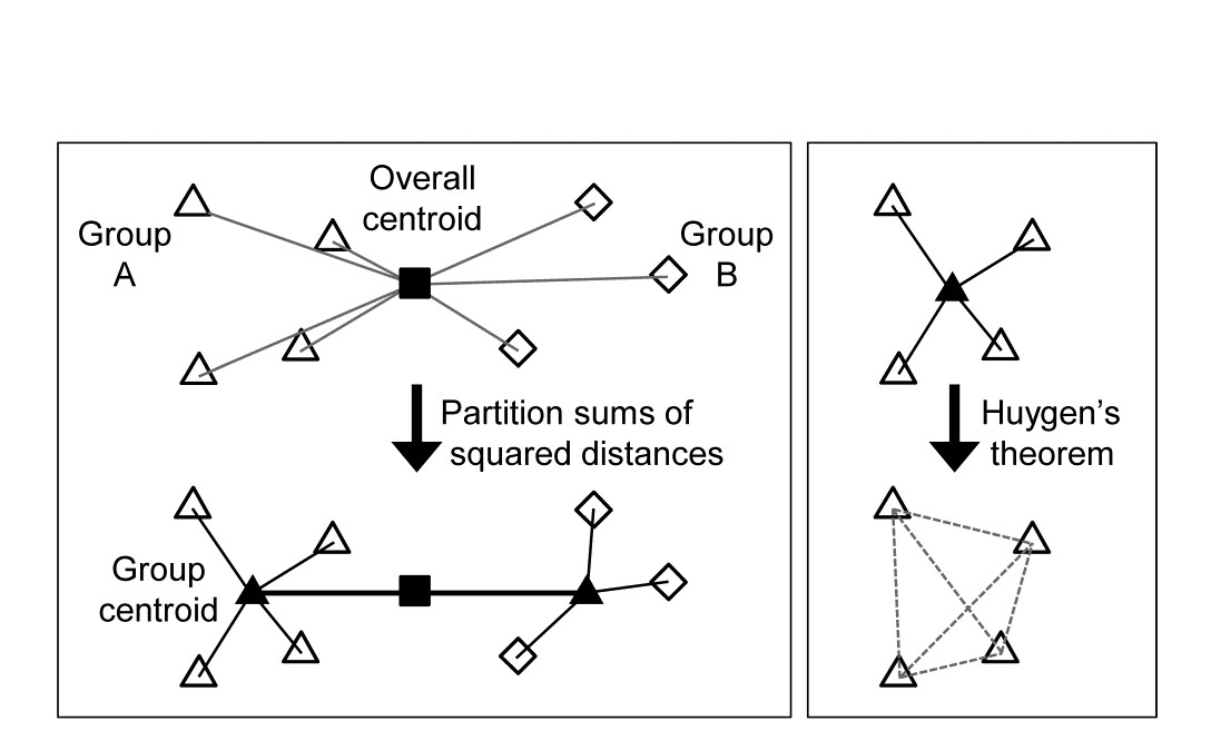
Fig. 3.8. Left: partitioning total sums of squared distances about centroid (d2) into within- and between-group d2. Right: within-group d2 determined by among-point d2, Huygen’s theorem.
There is a simple answer to this, a natural generalisation of the classic approach, met in equation (6.1), where we define the ANOSIM R statistic as:
$$ R = \frac{ \left( \overline{r} _ B - \overline{r} _ W \right) } { \frac{1}{2} M } \tag{3.1} $$
namely the difference between the average of the rank dissimilarities between the (two) groups and within the groups. This is suitably scaled by a divisor of M/2, where M = n(n-1)/2 is the total number of dissimilarities calculated between all the n samples currently being split. This divisor ensures that R takes its maximum value of 1 when the two groups are perfectly separated, defined as all between-group dissimilarities being larger than any within-group ones. R will be approximately zero when there is no separation of groups at all but this will never occur in this context, since we will be choosing the groups to maximise the value of R.
There is an important point not to be missed here: R is in no way being used as a test statistic, the reason for its development in Chapter 6 (for a test of no differences between a priori defined groups, R=0). Instead, we are exploiting its value as a pure measure of separation of groups of points represented by the high-dimensional structure of the resemblances (here perhaps Bray-Curtis, but any coefficient can be used with R, including Euclidean distance). And in that context it has some notable advantages: it provides the universal scaling we need of between vs. within group dissimilarities/distances (whatever their measurement scale) through their reduction to simple ranks, and this non-parametric use of dissimilarities is coherent with other techniques in our approach: non-metric MDS plots, ANOSIM and RELATE tests etc.
To recap: the binary divisive procedure starts with all samples in a single group, and if a SIMPROF test provides evidence that the group has structure which can be further examined, we search for an optimal split of those samples into two groups, maximising R, which could produce anything from splitting off a singleton sample through to an even balance of the sub-group sizes. The SIMPROF test is then repeated for each sub-group and this may justify a further split, again based on maximising R, but now calculated having re-ranked the dissimilarities in that sub-group. The process repeats until SIMPROF cannot justify further binary division on any branch: groups of two are therefore never split (see the earlier discussion).
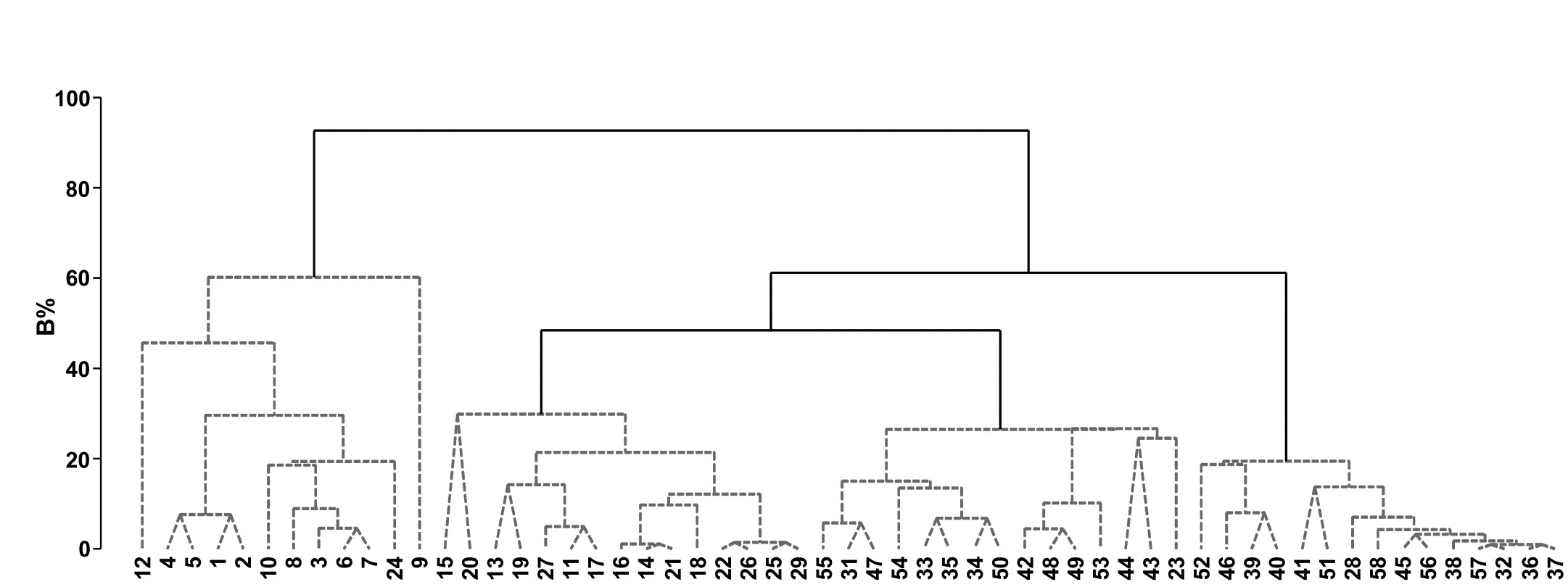
Fig. 3.9. Bristol Channel zooplankton {B}. Unconstrained divisive clustering of 57 sites (PRIMER’s UNCTREE routine, maximising R at each binary split), from Bray-Curtis on $\sqrt{} \sqrt{} $-transformed abundances. As with the agglomerative dendrogram (Fig. 3.7), continuous lines indicate tree structure which is supported by SIMPROF tests; this again divides the data into only four groups.
Bristol Channel zooplankton example
The tree diagram which results from the Bray-Curtis resemblances for the 57 Bristol Channel zooplankton samples is given in Fig 3.9. As with the comparative agglomerative clustering, Fig 3.7, it is convenient to represent all splits down to single points, but the grey dashed lines indicate divisions where SIMPROF provides no support for that sub-structure. Visual comparison of two such trees is not particularly easy, though they have been manually rotated to aid this (remember that a dendrogram is only defined down to arbitrary rotations of its branches, in the manner of a ‘mobile’). Clearly, however, only four groups have been identified by the SIMPROF tests in both cases, and the group constitutions have much in common, though are not identical. This is more readily seen from Figs. 3.10 a & b, which use a non-metric MDS plot (for MDS method see Chapter 5) to represent the community sample relationships in 2-d ordination space. These are identical plots, but demonstrate the agglomerative and divisive clustering results by the use of differing symbols to denote the 4 groups (A-D) produced by the respective trees. The numbering on Fig. 3.10a is that of the sites, shown in Fig. 3.2 (and on Fig. 3.10b the mean salinity at those sites, discretised into salinity scores, see equation 11.2). It is clear that only sites 9, 23 and 24 change groups between the two clustering methods and these all appear at the edges of their groups in both plots, which are thus reassuringly consistent (bear in mind also that a 2-d MDS plot gives only an approximation to the true sample relationships in higher dimensions, the MDS stress of 0.11 here being low but not negligible).
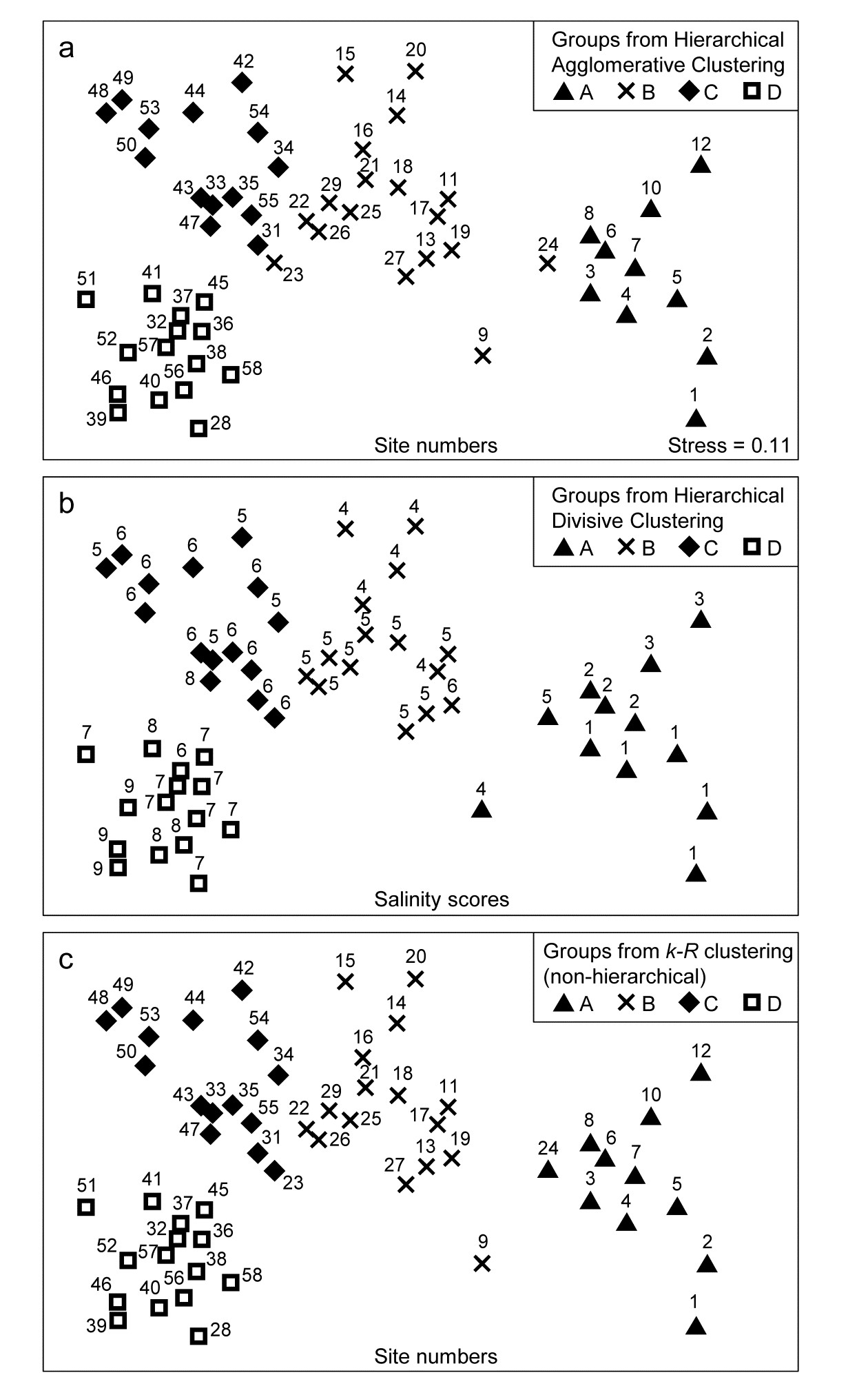
Fig. 3.10. Bristol Channel zooplankton {B}. Non-metric MDS ordination (Chapter 5) of the 57 sites, from Bray-Curtis on $\sqrt{} \sqrt{} $-transformed abundances. Symbols indicate the groups found by SIMPROF tests (four in each case, as it happens) for each of three clustering methods: a) agglomerative hierarchical, b) divisive hierarchical, c) k-R non-hierarchical. Sample labels are: a) & c) site numbers (as in Fig. 3.2), b) site salinity scores (on a 9-point scale, 1: <26.3, …, 9: > 35.1 ppt, see equation 11.2).
PRIMER v7 implements this unconstrained binary divisive clustering in its UNCTREE routine. This terminology reflects a contrast with the PRIMER (v6/ v7) LINKTREE routine for constrained binary divisive clustering, in which the biotic samples are linked to environmental information which is considered to be driving, or at least associated with, the community patterns. Linkage trees, also known as multivariate regression trees, are returned to again in Chapter 11. They perform the same binary divisive clustering of the biotic samples, using the same criterion of optimising R, but the only splits that can be made are those which have an ‘explanation’ in terms of an inequality on one of the environmental variables. Applied to the Bristol Channel zooplankton data, this might involve constraining the splits to those for which all samples in one sub-cluster have a higher salinity score than all samples in the other sub-cluster (better examples for more, and more continuous, environmental variables are given in Chapter 11 and Clarke, Somerfield & Gorley (2008) ). By imposing threshold constraints of this type we greatly reduce the number of possible ways in which splits can be made; evaluation of all possibilities is now viable so an iterative search algorithm is not required. LINKTREE gives an interesting capacity to ‘explain’ any clustering produced, in terms of thresholds on environmental values, but it is clear from Fig. 3.10b that its deterministic approach is quite likely to miss natural clusterings of the data: the C and D groups cannot be split up on the basis of an inequality on the salinity score (e.g. ≤6, ≥7) because this is not obeyed by sites 37 and 47.
For both the unconstrained or constrained forms of divisive clustering, PRIMER offers a choice of y axis scale between equi-spaced steps at each subsequent split (A% scale) and one which attempts to reflect the magnitude of divisions involved (B%), in terms of the generally decreasing dissimilarities between sub-groups as the procedure moves to finer distinctions. Clarke, Somerfield & Gorley (2008) define the B% scale in terms of average between-group ranks based on the originally ranked resemblance matrix, and that is used in Fig. 3.9. The A% scale generally makes for a more easily viewable plot, but the y axis positions at which identifiable groups are initiated cannot be compared.