16.7 Second-stage interaction plots
Phuket coral-reef times series
A rather different application of second-stage MDS¶ is motivated by considering the two-way layout from a time-series of coral-reef assemblages, along an onshore-offshore transect in Ko Phuket, Thailand {K}. These data were previously met in Chapter 15, where only samples from the earlier years 1983, 86, 87, 88 were considered (as available to Clarke, Warwick & Brown (1993) ). The time series was subsequently expanded to the 13 years 1983–2000, omitting 1984, 85, 89, 90 and 96, on transect A ( Brown, Clarke & Warwick (2002) ). The A transect consisted of 12 equally-spaced positions along the onshore-offshore gradient, and was subject to sedimentation disturbance from dredging for a new deep-water port in 1986 and 87. For 10 months during late 1997 and 98 there was also a wide scale sea-level depression in the Indian Ocean, leading to significantly greater irradiance exposures at mid-day low tides. Elevated sea temperatures were also observed (in 1991, 95, 97, 98), sometimes giving rise to coral bleaching events, but these generally resulted in only short-term partial mortalities.
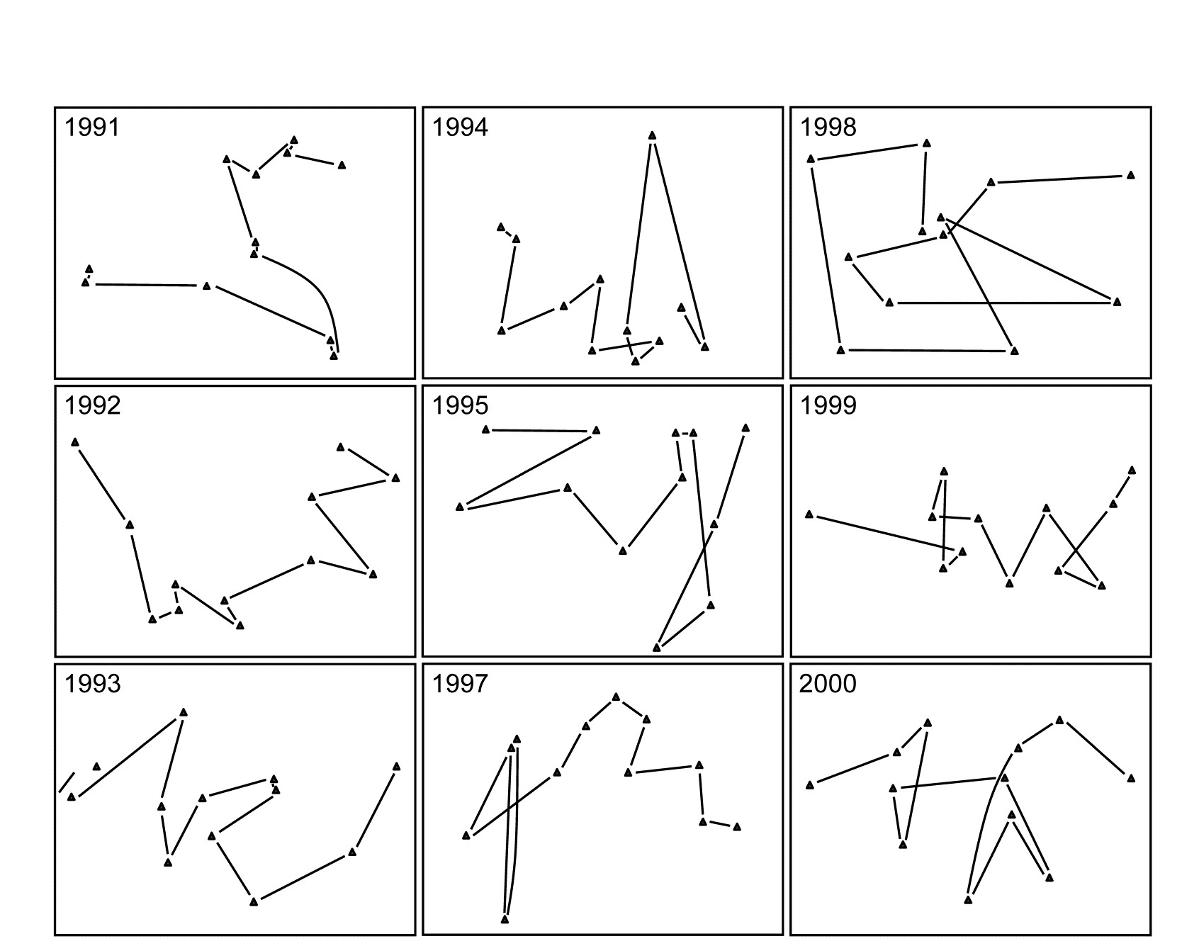
Fig. 16.12. Ko Phuket corals {K}. MDS plots of square-root transformed cover of 53 coral species for 12 positions (plotless line samples) on the A transect, running onshore to offshore, ordinated separately for each of 9 years (4 earlier years are shown in Fig. 15.6).
The two (crossed) factors here are the years and the positions along transect A (1-12, at the same spacing each year). Separate MDS plots of these 12 positions for each of the years 1983, 86, 87 and 88 were seen in Fig. 15.6 (first column). Fig. 16.12 adds nine more years (1991-95, 1997-2000) of the spatial patterns seen along the transect. The underlying resemblance matrices for each of these MDS plots can be matrix correlated, with the usual Spearman rank coefficient, in all possible pairs of years, giving a second-stage resemblance matrix (turned into a similarity by the transformation $50 (1 + \rho )$, if there are negative values). Input to a cluster analysis and nMDS, the result is Fig. 16.13a, which gives a clear visual demonstration of the years which are exceptional from the point of view of showing different patterns of reef assemblage turnover moving down the shore. The sedimentation-based disruption to the gradient in 1986 and 87, and the negative sea-level anomaly of 1998 seem both to be clearly identified. (There is however no statistical test that we can carry out on this second-stage matrix which would identify ‘significant’ change in those years, because in this simple two-way crossed design there is no replication structure to permit this). It is nonetheless interesting to note that the anomalous years are on opposite sides of the MDS plot, possibly suggesting that the departures from the ‘normal’ type of onshore-offshore gradient are of a different kind in 1998 than in 1986 & 87. Less speculative is the clear evidence from Fig. 16.13b that a comparable ‘first-stage’ nMDS plot does not obviously identify those years as anomalous. This is an ordination based on Bray-Curtis of ‘mean’ communities for each year, obtained by averaging the (square-root transformed) %cover values for each of the 53 coral species over the whole transect for each year.
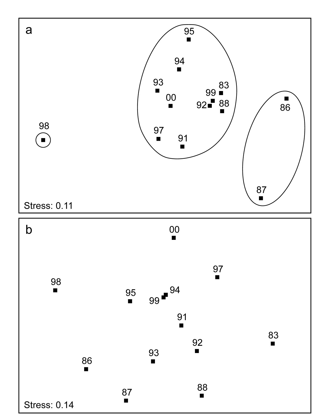
Fig. 16.13. Ko Phuket corals {K}. a) Second-stage MDS plot of 13 years in the period 1983 to 2000, based on comparing the multivariate pattern for each year of the 12 transect positions down the shore (transect A). Note the anomalous (non-seriated) patterns in 1986/7 and again in 1998, evidenced by the separation of these years on the plot and in the groups obtained from slicing a cluster dendrogram at a fixed similarity level. b) First-stage MDS of the whole assemblage in each year, by averaging the transformed cover matrix over transect positions.
Note the subtlety therefore of what a second-stage analysis is trying to isolate here. The compositions of the transect over the different years are not directly compared, as they are in a first-stage plot. There may (and will) be natural year-to-year fluctuations in area cover which would separate the transects on an MDS plot in which all transect positions and all years are displayed, but which do not disrupt the serial change in assemblage along the transect. The second-stage procedure will not be sensitive to such fluctuations. It eliminates them by concentrating only on whether the pattern is the same each year: assemblage similarities between the same transect points in different years do not enter the calculations at all (as observed in the schematic diagram for second-stage analysis of Fig. 16.4, where now each of the data matrices on the left represents the transect samples for a particular year). Disruptions to the (generally gradient) pattern in certain years are, in a sense, interactions between transect position and year, removing year-to-year main effects (by working only within each year) and it is such secondary, interaction effects that the second-stage MDS sets out to display.†
Clarke, Somerfield, Airoldi et al. (2006)
give the same analysis for the B transect and discuss two further applications, to Tees Bay data {t}, and a rocky shore colonisation study (see later).

Fig. 16.14. Schematic of the construction of a second-stage ‘interaction’ plot and test for a Before-After/Control-Impact design with (replicate) fixed sites from Impact and Control conditions sampled over several times Before and After an anticipated impact.
Before-After Control-Impact designs, over times
When there are sufficient sampling times in a study of the effects of an impact, both before and after that impact, and for multiple spatial replicates at both control and impact locations, the concept of a second-stage multivariate analysis may be a solution to one significant problem in handling such studies (known as ‘Beyond BACI’ designs, Underwood (1992) ), viz. how to allow for lack of independence in the communities observed when repeatedly returning to the same spatial patch. Monitoring communities at fixed locations (e.g. on permanent reef transects or over designated areas of rocky shore etc), in so-called repeated measures designs can sometimes be an efficient way of removing the effects of major spatial heterogeneity in the relevant habitat which would overwhelm any attempt at repeated random sampling, at each time, of different areas from the same general regions or treatment conditions under study. In other words, to detect smaller temporal change against a backdrop of large spatial variability could prove impossible without isolating the two factors, e.g. by monitoring the same area in space at different times, and different areas in space at the same time. A major imperative goes with this, however, and that is to recognise that the repeated measures (of community structure) in a single, restricted area, cannot in most cases be analysed as if they were independent§.
This is a problem that the second-stage multivariate analysis strategy neatly side-steps, because it has no need to invoke an assumption that the points making up a time course are in any way independent of each other: what ends up being compared is one whole time course with another (independent) time course, both resulting in single (independent) multivariate points in a second stage analysis. The above schema (Fig. 6.14) demonstrates the concept.
The data structure, on the left, shows the elements of a ‘Beyond BACI’ design‡, in which several areas (to call them fixed quadrats gives the right idea) will be sampled under both impact and reference (control) conditions, each quadrat being sampled at the same set of fixed times, which must be multiple occasions both before and after the impact is anticipated. It is the time courses of the multivariate community (seen here as MDS plots, but in reality the similarities that underlie these) which are then matched over quadrats in a second-stage correlation ($\rho$) matrix, shown to the right. This has a factor with two levels, control and impact, and replicate quadrats in each condition. A second-stage MDS plot from this second-stage similarity matrix would then show whether the temporal patterns differed for the two conditions, by noting whether the control and impacted quadrats clustered separately. A formal test for a significant effect of the impact is given by a 1-way ANOSIM on the second-stage similarity matrix. This is ‘on message’ with the purpose of a BACI design, namely to show (or not) that the temporal pattern under impact differs from that under control conditions, and we are justified in calling this an interaction test between B/A and C/I. In fact it is a rather general definition of interaction, entirely within the non-parametric framework that PRIMER adopts, and not at all in the same mould as the interaction term in a 2-way crossed ANOVA (or PERMANOVA) model, which is a strongly metric concept (see the discussion on page 6.17).
There are two strengths of this approach that can be immediately appreciated. Firstly, it is rare for control /reference sites to have the same Before assemblages as do the sites that will be part of the Impact group. For many studies, in order to find reference sites that will be outside the impact zone, one must move perhaps to a different estuary or coastal stretch, in which the natural assemblages will inevitably be a little different. Such initial differences are entirely removed however, in the above process - the only thing monitored and compared is the pattern of change over time within each site. Secondly, there is no suggestion here that assemblages at the sites (quadrats) will be independent observations from one time to the next. This is a repeated measures design, as previously alluded to. It is the whole time course of a quadrat, with all its internal autocorrelations among successive times, which becomes a single (multivariate) point in the final ANOSIM test, and all that is necessary for full validity of the test is that the quadrats should be chosen independently from each other, e.g. randomly and representatively across their particular conditions (C or I). This ability to compare whole temporal (or sometimes spatial) profiles as the experimental units of a design is certainly a viable approach to some ‘repeated measures’ data sets.
However, there are also some significant drawbacks. Using similarities only from within each quadrat will remove all differences in initial assemblage but will also remove differences in relative dispersion of the set of time trajectories. When control and impact sites do have similar initial assemblages, there will be no way of judging how far an impact site has moved from the control condition and whether it returns to that at some post-impact time; all that is seen is the extent to which the impact site reverts to its own initial state, before impact. Thus the second-stage process has inevitably ‘turned its back’ on the full information available in the species $\times$ samples matrix, to concentrate on only a small (though important) part, which might be considered a disadvantage. Also the simpler forms of BACI design in which there is only one time before and after the impact can clearly not be handled; there needs to be a rich enough set of times to be able to judge whether internal temporal patterns differ for control and impacted quadrats.
¶ Both applications of the second-stage idea are catered for in the PRIMER 2STAGE routine, the inputs either being a series of similarity matrices (which can be taken from any source provided they refer to the same set of sample labels), which is the use we have made of the routine so far, or a single similarity matrix, from a 2–way crossed layout with appropriately defined ‘outer’ and ‘inner’ factors (time and space, respectively, in this case so that patterns in space are matched up across times, or more often it will be the converse, matching up patterns in time across spatial layouts, so that space becomes the outer factor and time the inner). There can be no replication below each combination of inner and outer levels in the input similarity matrix, though levels of the outer factor might themselves encompass replication, by the ‘flattening’ of a 1-way layout of groups and replicates. An example will follow of a colonisation study in which replicate sites within treatments (which together make up the outer factor) are monitored through time (the inner factor).
† The idea also has close ties with the special form of ANOSIM test described in Chapter 6 (Fig. 6.9), with the ‘blocks’ as the outer year factor and the ‘treatments’ as the inner position factor, but instead of averaging the $\rho$ values in the final triangular matrix of that Fig. 6.9 schematic, we ordinate that matrix to obtain the second-stage MDS.
§ Unless the communities themselves are dynamic in the environment, so stochastic assumptions for the process being monitored replace randomness of sampling units for a fixed environment.
‡ Of course the samples are not entered into PRIMER in this rectangular form but by the usual entry of (say) rows as the species constituting the assemblages and columns as all the samples, but with factors defining Condition (levels of Control/Impact) and the unique Quadrat number which identifies that fixed quadrat over time, and a factor giving the sampling Time (with matching levels for all quadrats). The 2STAGE routine is then entered with the outer factor Quadrat and the inner factor Time, resulting in a resemblance matrix among all quadrats, in terms of their patterns though time. This has a 1-way structure of Condition (C/I) and replicate quadrats within each condition, input to ANOSIM.