6.6 Example: Clyde nematodes (2-way nested case)
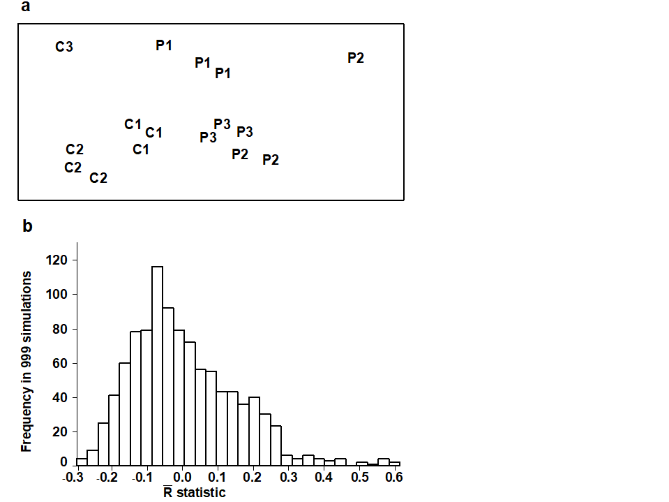
Lambshead (1986) analysed meiobenthic communities from three putatively polluted (P) areas of the Firth of Clyde and three control (C) sites, taking three replicate samples at each site (with one exception). The resulting MDS, based on fourth-root transformed abundances of the 113 species in the 16 samples, is given in Fig. 6.6a. The sites are numbered 1 to 3 for both conditions but the numbering is arbitrary – there is nothing in common between P1 and C1 (say). This is what is meant by sites being ‘nested within conditions’. Two hypotheses are then appropriate:
H1: there are no differences among sites within each treatment (control or polluted conditions);
H2: there are no differences between control and polluted conditions.
The approach to H2 might depend on the outcome of testing H1.
H1 can be examined by extending the 1-way ANOSIM test to a constrained randomisation procedure. The presumption under H1 is that there may be a difference between general location of C and P samples in the multivariate space (as approximately viewed in the MDS plot) but within each condition there cannot be any pattern in allocation of replicates to the three sites. Treating the two conditions entirely separately, one therefore has two separate 1-way permutation analyses of exactly the same type as for the Frierfjord macrofauna data (Fig. 6.3). These generate test statistics $R_C$ and $R_P$, computed from equation (6.1), which can be combined to produce an average statistic $\overline{R}$. This can be tested by comparing it with $\overline{R}$ values from all possible permutations of sample labels permitted under the null hypothesis. This does not mean that all 16 sample labels may be arbitrarily permuted; the randomisation is constrained to take place only within the separate conditions: P and C labels may not be switched. Even so, the number of possible permutations is large (around 20,000).
Notice again that the test is not restricted to balanced designs, i.e. those with equal numbers of replicate samples within sites and/or equal numbers of sites within treatments (although lack of balance causes a minor complication in the efficient averaging of $R_C$ and $R_P$, see Clarke (1988) and Clarke (1993) ). Fig. 6.6b displays the results of 999 simulations (constrained relabellings) from the permutation distribution for $\overline{R}$ under the null hypothesis H1. Possible values range from –0.3 to 0.6, though 95% of the values are seen to be <0.27 and 99% are <0.46. The observed $\overline{R}$ of 0.75 therefore provides a strongly significant rejection of hypothesis H1.
Fig. 6.6. Clyde nematodes {Y}. a) MDS of species abundances from three polluted (P1-P3) and three control sites (C1–C3), with three replicate samples at most sites (stress = 0.09). b) Simulated distribution of the test statistic $\overline{R}$ under the hypothesis H1 of ‘no site differences’ within each condition; the observed $\overline{R}$ is 0.75.
H2, which will usually be the more interesting of the two hypotheses, can now be examined. The test of H1 demonstrated that there are, in effect, only three genuine replicates (the sites 1-3) at each of the two conditions (C and P).
This is a 1-way layout, and H2 can be tested by 1-way ANOSIM but one first needs to combine the information from the three original replicates at each site, to define a similarity matrix for the 6 new ‘replicates’. Consistent with the overall strategy that tests should only be dependent on the rank similarities in the original triangular matrix, averages are first taken over the appropriate ranks to obtain a reduced matrix. For example, the similarity between the three P1 and three P2 replicates is defined as the average of the nine inter-group rank similarities; this is placed into the new similarity matrix along with the 14 other averages (C1 with C2, P1 with C1 etc) and all 15 values are then re-ranked; the 1-way ANOSIM then gives R = 0.74. There are only 10 distinct permutations so that, although this is actually the most extreme R value possible in this case, H2 is only able to be rejected at a p<10% significance level.
The other scenario to consider is that the first test fails to reject H1. There are then two possibilities for examining H2:
a) Proceed with the average ranking and re-ranking exactly as above, on the assumption that even if it cannot be proved that there are no differences between sites it would be unwise to assume that this is so; the test may have had rather little power to detect such a difference.
b) Infer from the test of H1 that there are no differences between sites, and treat all replicates as if they were separate sites, e.g. there would be 7 replicates for control and 9 replicates for polluted conditions in a 1-way ANOSIM test applied to the 16 samples in Fig. 6.6a.
Which of these two courses to take is a matter for debate, and the argument here is exactly that of whether “to pool or not to pool” in forming the residual for the analogous univariate 2-way ANOVA. Option b) will certainly have greater power but runs a real risk of being invalid; option a) is the conservative test and it is certainly unwise to design a study with anything other than option a) in mind.
¶ Note that the ANOSIM program in the PRIMER package always takes the first of these options, so if the second option is required the resemblance matrix needs to be put through ANOSIM again, this time as a 1-factor design with the combined factor of condition and site (6 levels, C1, C2, C3, P1, P2, P3 and 3 replicates within most of these levels).

